Skip to content

Differentiable simulation: Diffrax adjoint pass-through, tests, and an Orszag-Tang inverse-design example - #44

Open
rogeriojorge wants to merge 9 commits into
mainfrom
agent/autodiff-plan
Open

rogeriojorge wants to merge 9 commits into
mainfrom
agent/autodiff-plan

Conversation

@rogeriojorge

@rogeriojorge rogeriojorge commented Sep 13, 2026 •

Copy link
Copy Markdown
Member

Target: main. Head: 3ad4a9d. Old head: 49c4c69, a merge of #21/#18/#13 and other branches carrying about 950 lines of unrelated diff.

Stacked on #50 (2744422), which provides max_steps, throw and the validity metadata. Until #50 merges, this diff shows #50's four commits. Review only the top two:

This PR does not depend on #13, #18 or #21.

Change

  • simulation accepts adjoint and progress_meter, both static.
    • adjoint defaults to RecursiveCheckpointAdjoint(), so behaviour is unchanged.
    • RecursiveCheckpointAdjoint(checkpoints=k) bounds reverse-mode memory.
    • ForwardMode() works with jax.jacfwd.
  • kinetic_energy_species is returned real, so scalar objectives are real.
  • Examples/2D_Orszag_Tang_optimization.py: the controls are stream-function phases and the objective is magnetic-energy conversion. It checks the reverse-mode gradient against centred differences, then runs L-BFGS-B.
    • The example no longer keeps its own real-FFT weights. It had w = 1 for k=0 and w = 2 otherwise, a second, parity-dependent copy of the Parseval rule that Fix odd-grid RFFT energy weights; add a Hermite boundary diagnostic #9 fixes in the library.
    • It now takes the grid mean of Bx² + By² after irfftn, which needs no weights for any Nx.
    • The example is not run in CI.

AD contract

  • Supported: reverse mode through Diffrax's checkpointed adjoint, and forward mode, for explicit solvers such as Dopri8 (adaptive) and Tsit5 (fixed step).
  • Not supported: ImplicitMidpoint in reverse mode. Its Newton loop is a lax.while_loop.
  • Objectives must be real scalars.

Tests (local, macOS CPU, Python 3.12, jax 0.11.2, diffrax 0.7.2, at 3ad4a9d)

  • python -m pytest -q -n 2 tests: 18 passed. The autodiff file alone takes 17 s on 2 workers.
  • JAX_ENABLE_X64=1 python -m pytest -q -n 2 tests/test_autodiff.py: 6 passed.

tests/test_autodiff.py uses a tiny two-species Orszag–Tang case (8², 4³ Hermite):

  • reverse mode = forward mode (rtol 1e-9) = finite differences, adaptive Dopri8;
  • the gradient does not depend on the checkpoint budget (1, 4, 20);
  • reverse-pass workspace does not grow from 10 to 80 steps;
  • current-density and time-window objectives.
  • New, finite-difference plateau: centred differences of a real scalar along a fixed direction, eps = 1e-1 … 1e-7.
    • The error relative to the AD directional derivative falls by more than 50× from eps 1e-2 to 1e-3.
    • It stays below 1e-6 over at least three consecutive eps.

Example: python Examples/2D_Orszag_Tang_optimization.py --t-max 5 --iterations 2

  • reverse vs centred differences: max relative difference 2.9e-8;
  • L-BFGS-B: 0.99956 → 0.991404 in 2 iterations;
  • 9.9 s wall time.

GitHub CI: see the checks on this head. The local results above are not CI results.

Owner decision

Review the final API and gradient contract once:

  • adjoint and progress_meter as static simulation arguments;
  • real kinetic energies.

@codecov

codecov Bot commented Sep 13, 2026 •

Copy link
Copy Markdown

Codecov Report

✅ All modified and coverable lines are covered by tests.

Files with missing lines Coverage Δ
spectrax/_diagnostics.py 73.86% <100.00%> (ø)
spectrax/_simulation.py 100.00% <100.00%> (ø)

... and 1 file with indirect coverage changes

🚀 New features to boost your workflow:
  • ❄️ Test Analytics: Detect flaky tests, report on failures, and find test suite problems.

@rogeriojorge

Copy link
Copy Markdown
Member Author

Phase 1a: evidence for the first CPU showcase runs

The files are on the evidence branch at 87685b9. These are 32²×4³ runs, so they are not resolution-validated yet; that is Phase 2a, now running. The figures come from Examples/2D_Orszag_Tang_optimization.py at 9600144 on an Apple M3 Max CPU.

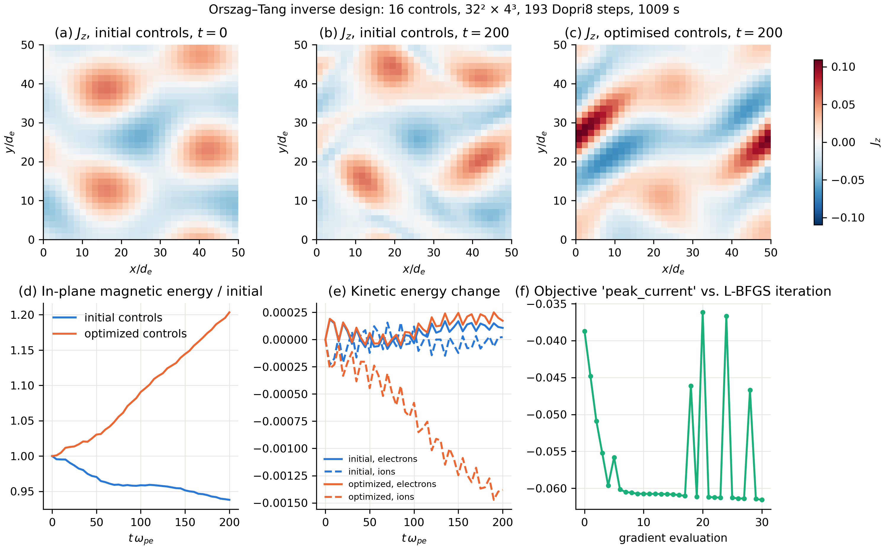
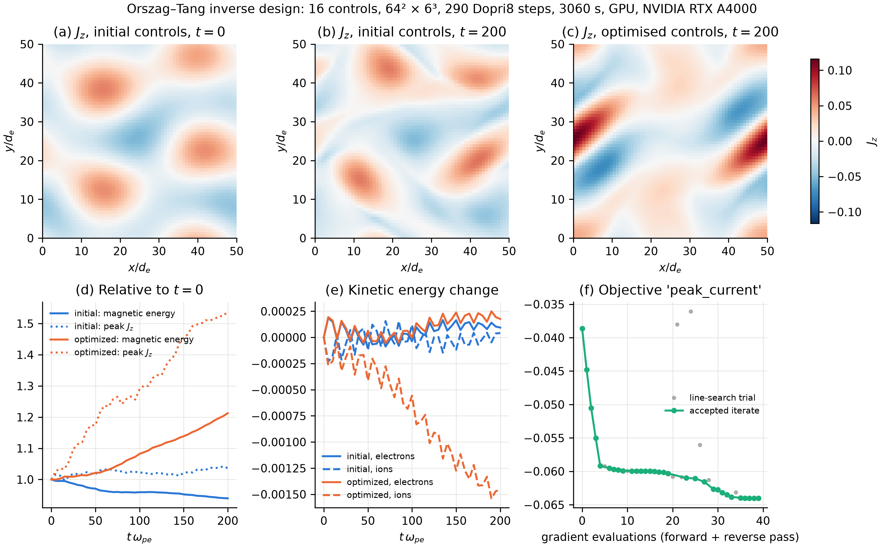
Current-sheet intensification (peak_current). The smooth peak of Jz at T=200 rises from 0.0387 to 0.0616. The initial peak is unchanged (0.0373 vs 0.0374), so the gain is dynamical. Jz intensifies 1.65× instead of 1.04×, the in-plane magnetic energy grows 20 %, and ion flow energy drops by 1.4e-3.

peak current

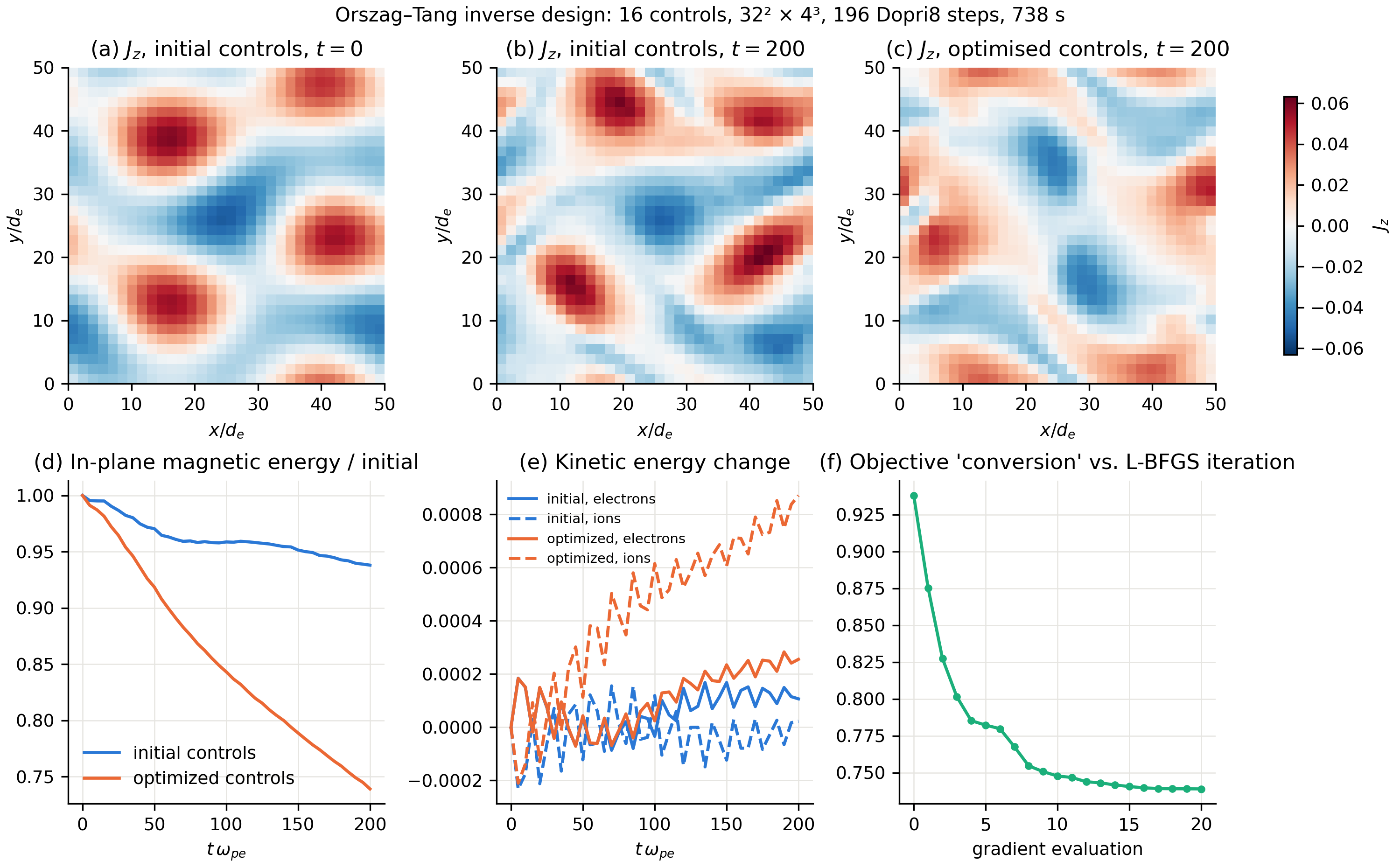
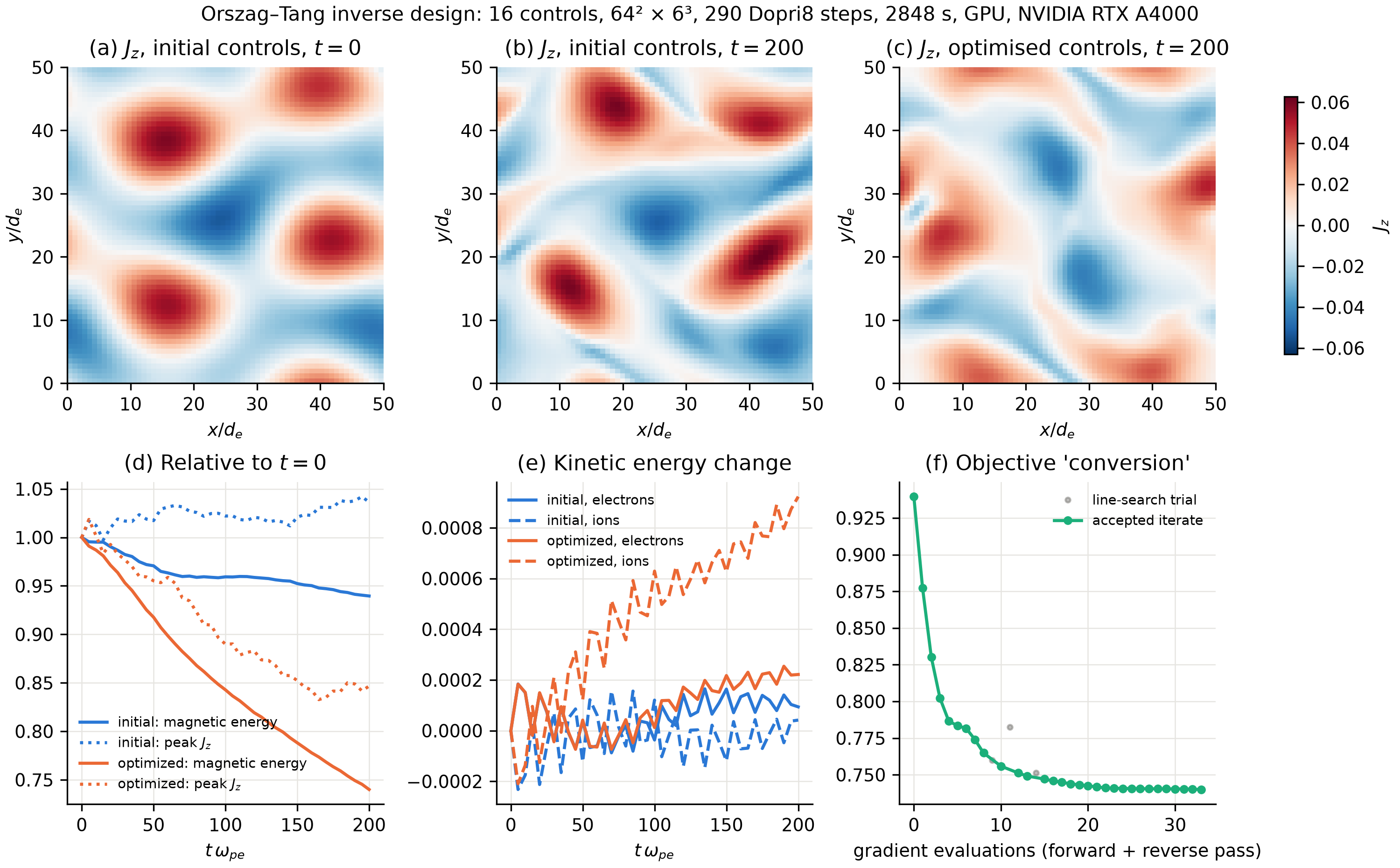
Magnetic-energy conversion (conversion). The fraction of in-plane magnetic energy converted by T=200 rises from 6.2 % to 26.1 %. The ion kinetic-energy gain is 39× the baseline. The energy-weighted mean k² falls from 3.83 to 3.53, so the optimiser did not simply push energy to dissipative small scales.

conversion

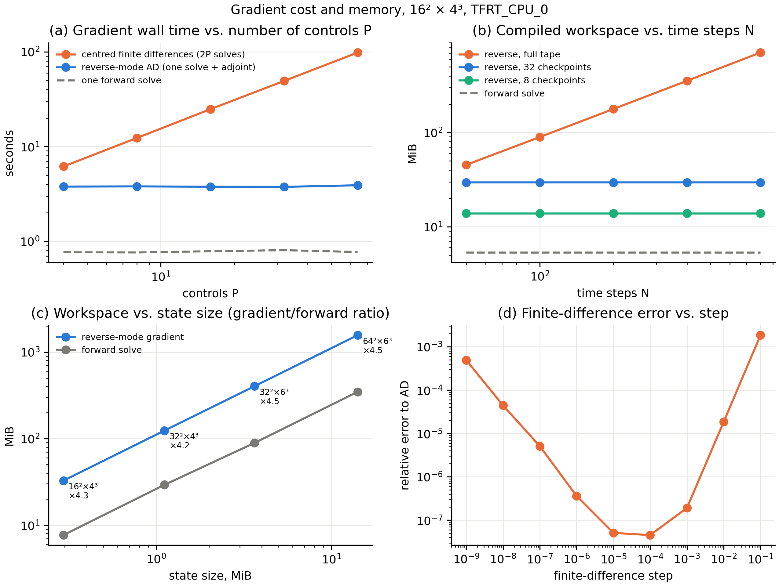
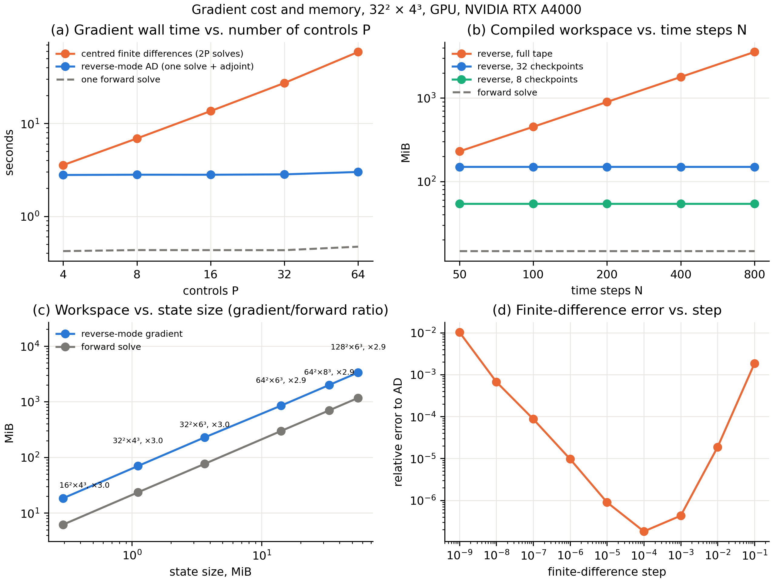
Gradient cost and memory. The AD gradient costs about 5 forward solves at every P, while FD is 1.6× (P=4) to 25× (P=64) slower. The reverse-pass workspace is flat in N with checkpointing and linear with a full tape. The gradient/forward workspace ratio stays at 4.2–4.5× from 16²×4³ to 64²×6³.

benchmark

Two figure fixes follow in the next commit. The objective panels will plot accepted L-BFGS iterates instead of line-search trial points (the spikes in the peak_current history). The device label will name the processor. PDFs are next to the PNGs.

@rogeriojorge

Copy link
Copy Markdown
Member Author

Phase 2a gate: passed

The initial and optimised controls from the 32²×4³ runs were frozen and re-evaluated at higher resolution: forward solves only, adaptive Dopri8, T=200. Raw JSON is on the evidence branch at 9e1a89a. CPU: Apple M3 Max. GPU: RTX A4000.

Relative change of the objective, optimised vs initial controls:

objective 32²×4³ (trained) 32²×6³ 64²×4³ 64²×6³ 64²×8³ 128²×6³ 64²×6³, tolerance 1e-9
conversion −21.2 % −21.2 % −21.2 % −21.2 % −21.2 % −21.2 % −21.2 %
peak_current −59.1 % −57.1 % −59.5 % −57.4 % −57.7 % −57.4 % −57.4 %

Gate criteria:

  • Retained improvement: pass. The optimised controls win at every resolution. conversion keeps 100 % of its gain and peak_current keeps 97 % at 64²×6³, 64²×8³ and 128²×6³.
  • Energy error: pass, with a tighter tolerance. The relative total-energy error at T is Dopri8 time-integration error, and it grows with grid size at tolerance 1e-7:
grid tolerance 1e-7 tolerance 1e-9
32² 1e-9 4e-11
64² 3–5e-6 1e-10
128² 1–2e-4 not run

At 64²×8³ it is 1e-12 even at 1e-7, because the stiffer system forces smaller steps. The objective values change by at most 0.05 % between tolerances 1e-7 and 1e-9. Phase 3 therefore runs at tolerance 1e-9.

Physics read-out (consistent across resolutions):

  • conversion sends the extra converted magnetic energy mostly to ions: +8.7e-4 against +2.2e-5 at baseline.
  • peak_current intensifies Jz 1.6× by drawing on ion flow energy, while the in-plane field grows 20 %.
  • In both runs the initial peak current and spectral centroid are essentially unchanged, so the gains come from the nonlinear evolution, not from a rearranged initial state.

@rogeriojorge

rogeriojorge commented Sep 13, 2026 •

Copy link
Copy Markdown
Member Author

Phase 2c: phase-only controls (--fixed-amplitudes)

With only the 8 phases free, every mode's magnetic energy, current spectrum and drift energy is fixed. Settings are otherwise as in the first runs: 32²×4³, T=200, CPU, commit 8380edc. Both runs converged, meeting L-BFGS-B's projected-gradient tolerance within 20 iterations. Files are on the evidence branch at abd99e0.

baseline 16 controls (amplitudes + phases) 8 phase-only controls
conversion: in-plane magnetic energy converted by T 6.2 % 26.1 % 23.9 %
conversion: ion kinetic-energy gain 2.2e-5 8.7e-4 7.6e-4
peak_current: objective (smooth peak of Jz at T) 0.0387 0.0616 0.0614
peak_current: Jz peak at t=0 0.0373 0.0374 0.0493
peak_current: dynamical intensification Jz(T)/Jz(0) 1.04× 1.65× 1.25×

Conversion. Linear evolution on the uniform background cannot change any mode's energy, so the phase-only gain is pure nonlinear coupling. It reaches 89 % of the full-control improvement. This is the cleanest statement of the showcase: with the same initial energy in every Fourier mode, the arrangement of the modes alone controls how much magnetic energy the vortex converts, and a gradient finds it.

Peak current. The p-norm objective depends on phases already at t=0. Phase-only control reaches the same objective partly by building a larger initial peak (0.049 against 0.037), and its dynamical intensification (1.25×) is below the full-control run (1.65×). For current-sheet formation, the full-control result, with an unchanged initial peak, remains the showcase. The phase-only run is reported as a caveat.
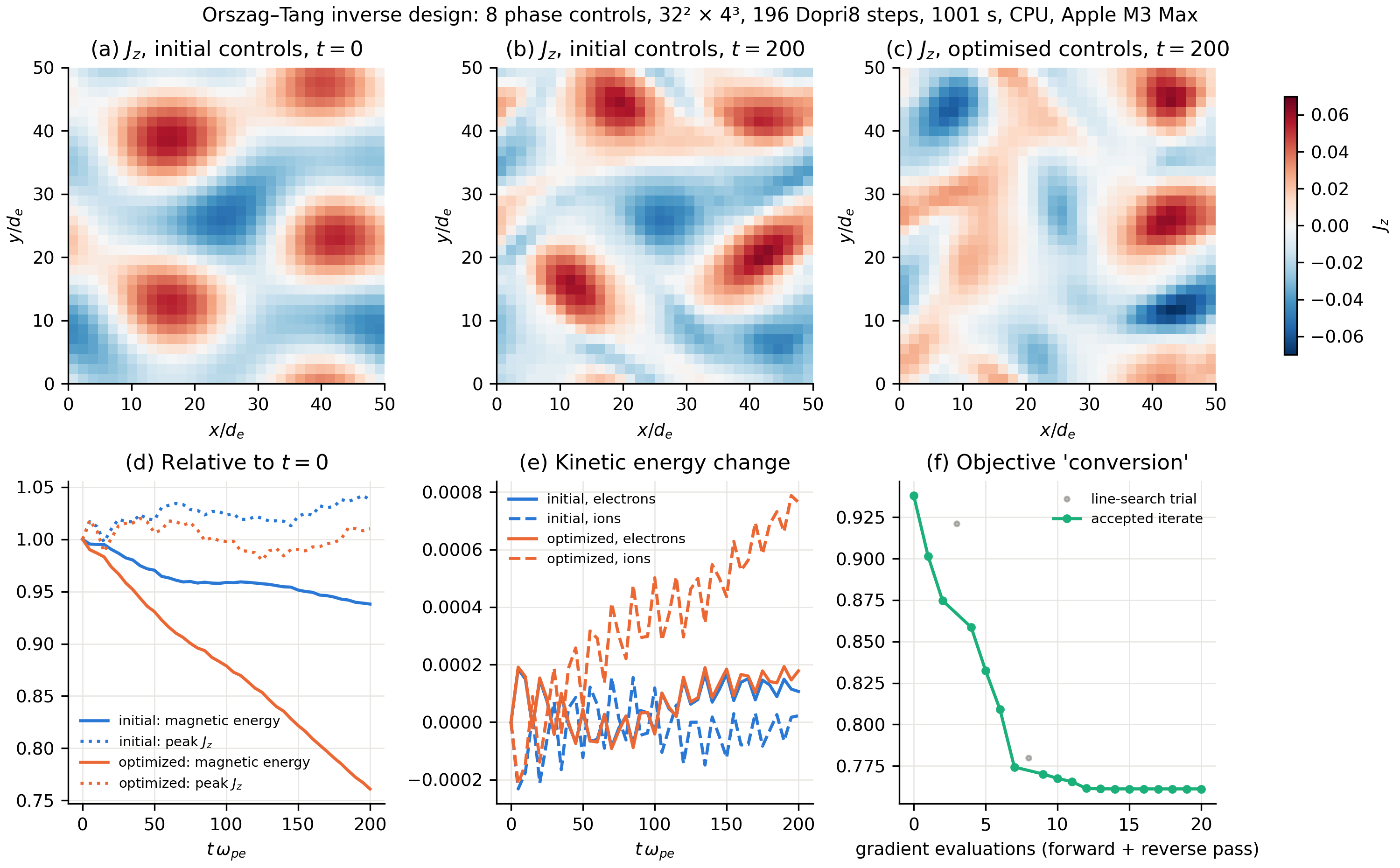
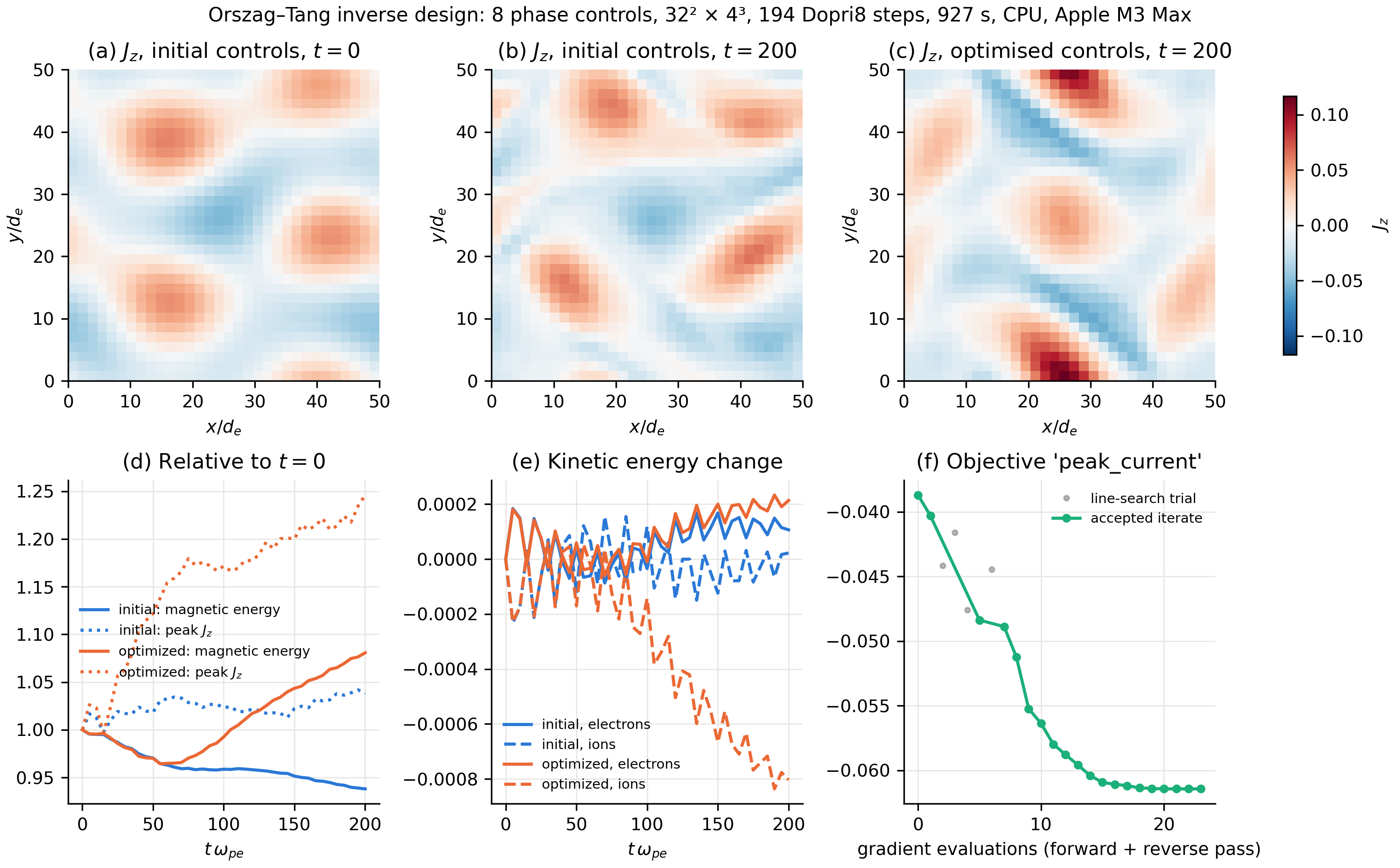
conversion, phase-only

peak current, phase-only

Provenance note: the phase-only conversion report records commit 8380edc, but that process imported the example at 620fd14. Provenance was captured when the report was written, not at the start of the run; this is fixed on the PR branch. The optimisation path is numerically identical between the two commits, so the result is unaffected. Its figure was re-plotted from the JSON to pick up the title fix.

@rogeriojorge

Copy link
Copy Markdown
Member Author

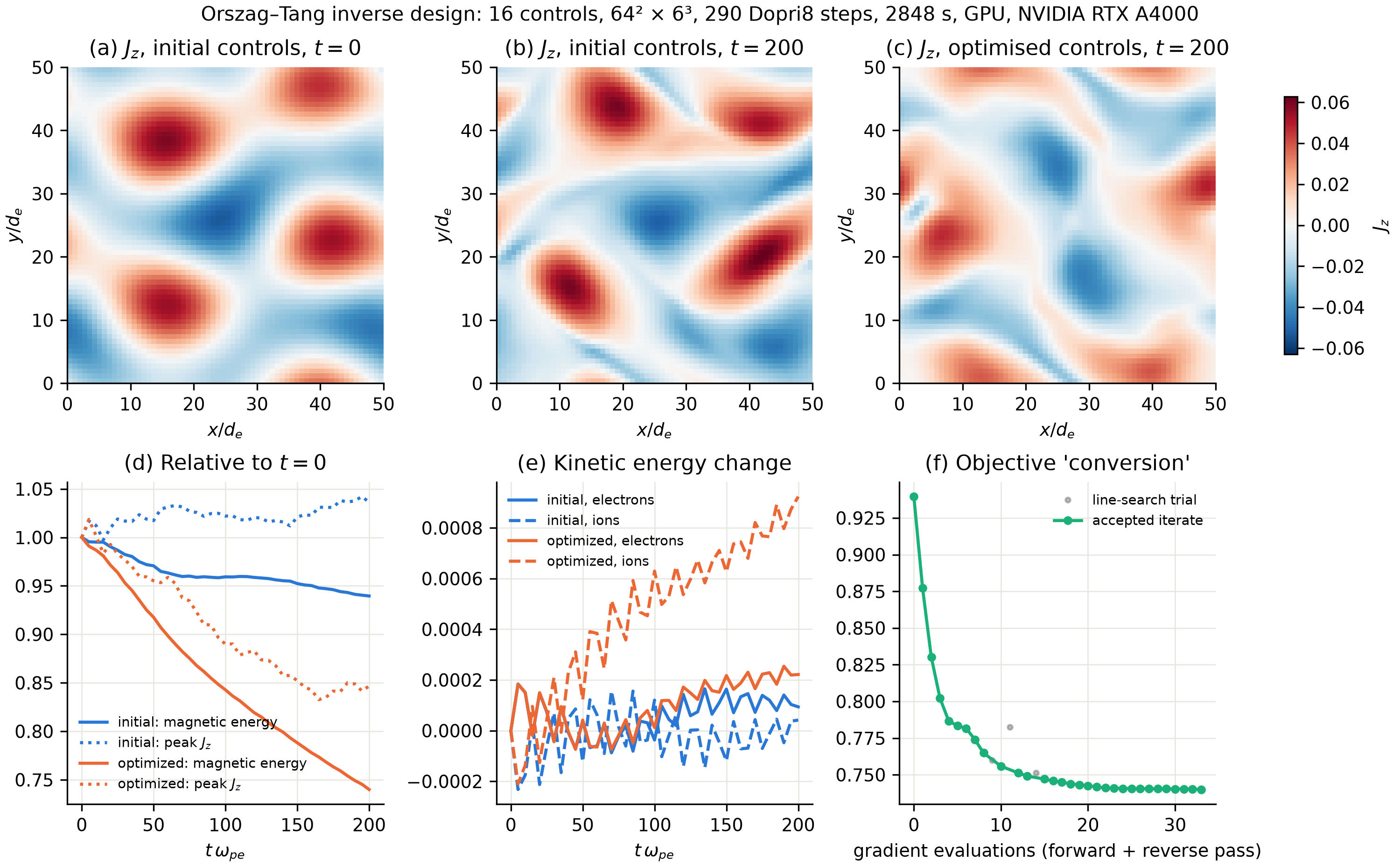
Phase 3a/3b: conversion at 64²×6³ on one RTX A4000

Settings. 16 controls, T=200, adaptive Dopri8 at tolerance 1e-9, 32 checkpoints, commit 8380edc. Files are on the evidence branch at 4ec9acb.

initial controls optimised controls
objective: in-plane magnetic energy at T / initial 0.940 0.740
magnetic energy converted by T 6.0 % 26.0 %
electron kinetic-energy gain 9.4e-5 2.2e-4
ion kinetic-energy gain 4.2e-5 9.2e-4
Dopri8 steps 277 290

Cost. 30 L-BFGS-B iterations (the cap) used 34 gradient evaluations at 77 s each, for 47.5 min in total including 95 s of compilation. The optimum matches the 32²×4³ CPU run (0.938 → 0.739), so the low-resolution search already found the physical optimum.

Validation (3b). Frozen optimised controls, tolerance 1e-9:

resolution initial → optimised change energy error at T
64²×8³ 0.9409 → 0.7409 −21.3 % 7e-11
128²×6³ 0.9396 → 0.7400 −21.2 % 1.0–1.4e-8

conversion 64x6 GPU

Scope change for the rest of Phase 3.

  • The job was not stalled; the peak-current optimisation is running normally (76.8 s per gradient evaluation).
  • Because the low-resolution optimum already transfers, the remaining GPU work was trimmed. The GPU benchmark now stops at P=64 controls and N=800 steps instead of P=128 and N=1600, saving roughly 25 min of finite-difference and 1600-step-tape work. The CPU benchmark already shows both scaling trends.
  • Peak-current validation and the per-process peak-memory sweep are unchanged.

@rogeriojorge

Copy link
Copy Markdown
Member Author

Phase 3 complete, and the publication figures (4a)

All numbers are from one NVIDIA RTX A4000 in float64 at commit 8380edc. Plotting fixes that came later do not change any result. Raw JSON, logs, PNGs and PDFs are on the evidence branch at 5fe62bf.

Figure 1 (main): magnetic-energy conversion by design

Figure 1

Caption. Gradient-based inverse design of the 2D Orszag–Tang vortex.

  • Controls. The amplitudes and phases of the 8 lowest Fourier modes of the in-plane magnetic stream function (16 controls), at fixed in-plane magnetic energy. Electrons carry the consistent out-of-plane current.
  • Panels. (a) J_z at t=0 for the reference field. (b) J_z at t ω_pe=200 for the reference field. (c) J_z at t ω_pe=200 for the field that minimises the in-plane magnetic energy remaining at that time. (d) In-plane magnetic energy (solid) and smooth peak of J_z (dotted), relative to t=0. (e) Change in electron (solid) and ion (dashed) kinetic energy. (f) Objective against gradient evaluations; grey points are rejected line-search trials.
  • Setup. 64²×6³ Fourier–Hermite resolution, two species, m_i/m_e=25, ν=1, adaptive Dopri8 at tolerance 1e-9. 30 L-BFGS-B iterations took 47.5 min.
  • Result. The optimised field converts 26.0 % of the in-plane magnetic energy by t ω_pe=200, against 6.0 % for the reference, and mostly heats the ions. The result is unchanged at 64²×8³ and 128²×6³. With only the phases free, every mode energy is fixed and the gain still reaches 89 % of this value, so the effect is nonlinear.

Figure 2 (methods): cost and memory of gradients

Figure 2

Caption. Cost and memory of reverse-mode gradients through SPECTRAX, 32²×4³, T=100.

  • (a) Wall time of one gradient against the number of controls P. Reverse-mode AD is one forward solve plus a checkpointed reverse pass; centred finite differences are 2P forward solves; the dashed line is one forward solve.
  • (b) Compiled reverse-pass workspace against the number of fixed time steps N, for a full trajectory tape and for 8 and 32 checkpoints.
  • (c) Compiled workspace of a forward solve and a gradient against state size, from 16²×4³ to 128²×6³ with 8 checkpoints; labels give the gradient/forward ratio.
  • (d) Relative error of the finite-difference gradient against the AD gradient, as a function of step size.
controls P 4 8 16 32 64
AD gradient, s (forward solve ≈ 0.43 s) 2.79 2.81 2.80 2.83 3.00
centred FD gradient, s 3.56 6.89 13.6 27.3 58.9
FD / AD 1.3× 2.5× 4.8× 9.6× 19.6×

Peak device memory, one process per row (adaptive Dopri8, T=20):

resolution state forward gradient, 8 checkpoints ratio gradient, 32 checkpoints ratio gradient time, 8 / 32 checkpoints
32²×4³ 1.1 MiB 64 MiB 176 MiB 2.75× 258 MiB 4.0× 0.51 s / 0.44 s
64²×6³ 14.1 MiB 311 MiB 862 MiB 2.77× 1907 MiB 6.1× 6.2 s / 5.3 s
64²×8³ 33.2 MiB 731 MiB 2112 MiB 2.89× 4514 MiB 6.2× 22.4 s / 19.5 s
128²×6³ 55.6 MiB 1226 MiB 3408 MiB 2.78× 7523 MiB 6.1× 67.6 s / 51.7 s

With 8 checkpoints a gradient needs a fixed 2.8–2.9× the memory of a forward solve at every resolution. Its compiled workspace stays at 54 MiB for 50 to 800 steps, whereas a full tape grows from 230 MiB to 3.6 GiB. More checkpoints trade memory for less recomputation. The earlier 128²×6³ out-of-memory error came from a GPU shared with another job, not from the method.

Supplementary figure S1: current-sheet intensification

Figure S1

Caption. The layout and setup match Figure 1, with the objective changed to the smooth peak (p=8 norm) of J_z at t ω_pe=200.

  • Result. The optimised peak is 0.0640 against 0.0386 for the reference, +66 %, unchanged at 64²×8³ and 128²×6³. Forty gradient evaluations took 51 min.
  • Mechanism. The in-plane magnetic energy grows by 21 % while the ions lose kinetic energy.
  • Caveat. Part of the gain comes from a rearranged initial field: the initial peak rises from 0.0373 to 0.0416. The dynamical intensification is 1.54× against 1.04× for the reference.

Validation of both optima (3b), tolerance 1e-9

resolution conversion energy error at T peak_current energy error at T
64²×6³ (trained) 0.9396 → 0.7400 (−21.2 %) 1.4e-10 0.0386 → 0.0640 (+65.7 %) 1.4e-10
64²×8³ 0.9409 → 0.7409 (−21.3 %) 7.2e-11 0.0386 → 0.0640 (+65.7 %) 3.6e-11
128²×6³ 0.9396 → 0.7400 (−21.2 %) 1.4e-8 0.0386 → 0.0640 (+65.7 %) 1.3e-8

The draft methods paragraph and captions are kept with the evidence under paper/ and follow these numbers.

@rogeriojorge

Copy link
Copy Markdown
Member Author

Phase 5: time-window objectives, parameter sensitivities, and the DG driver

5c: sensitivity of the optimised designs to physical parameters

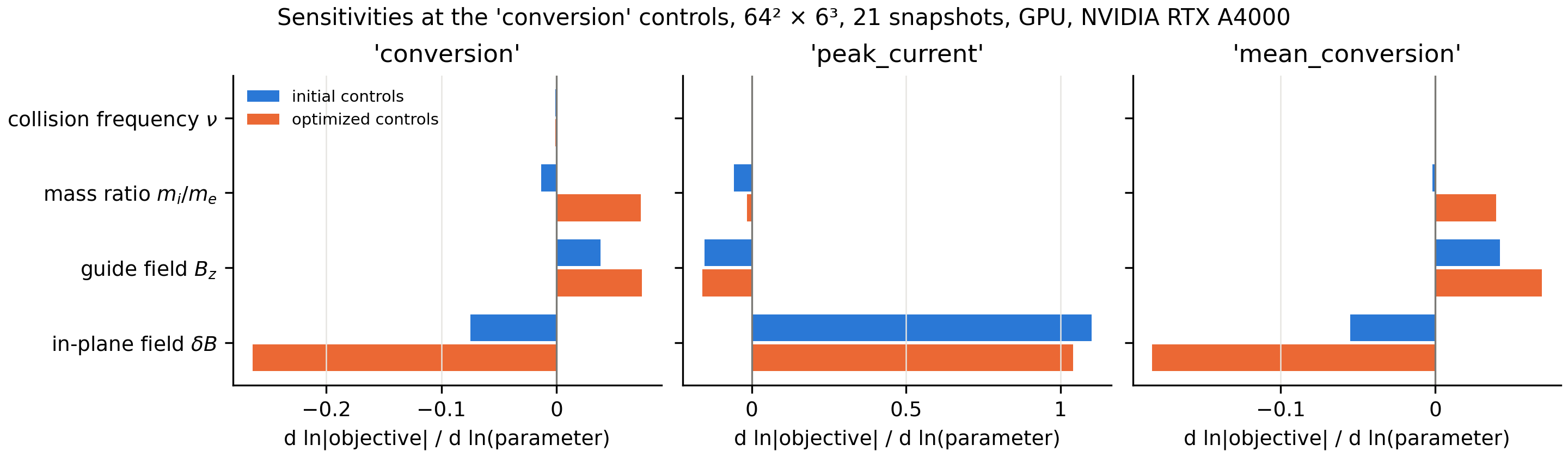
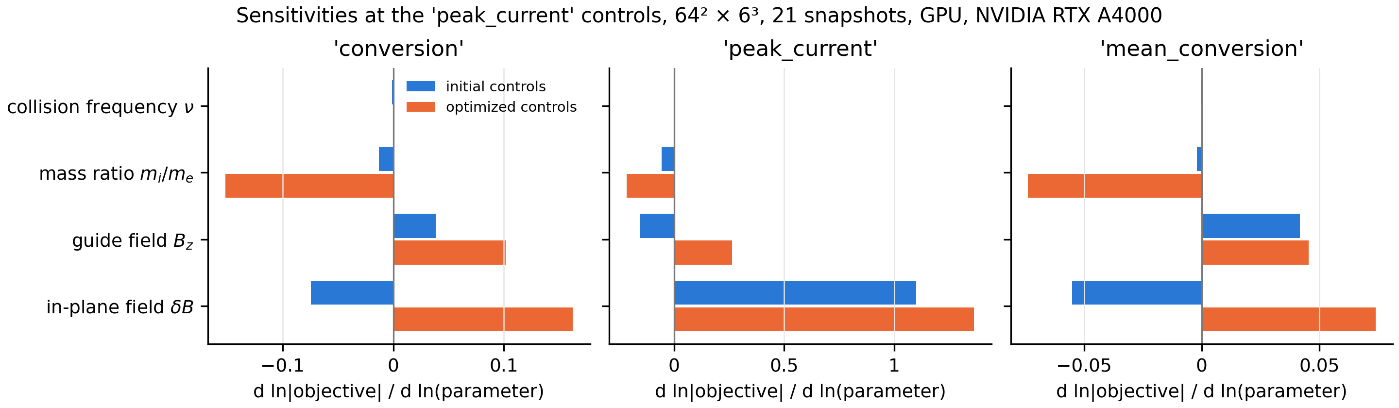
The new sensitivity mode differentiates every objective with respect to four physical parameters: collision frequency ν, mass ratio m_i/m_e, guide field B_z and in-plane field amplitude δB. It uses forward mode, jax.jacfwd with adjoint=ForwardMode(), which propagates four tangents through one adaptive Dopri8 solve.

  • Setup. 64²×6³, tolerance 1e-9, 21 saved snapshots, one RTX A4000, commit 3ce58b2.
  • Cost. Each control set took 96–120 s, including compilation.
  • Accuracy. Every entry matches centred finite differences within 4.4e-6 in log-sensitivity units.
  • Files. Evidence at dfd5399.

Logarithmic sensitivity d ln|J| / d ln p of each objective at the reference controls and at its own optimum:

parameter conversion, reference conversion, its optimum peak_current, reference peak_current, its optimum
collision frequency ν −0.0009 −0.0011 +0.00002 +0.0036
mass ratio m_i/m_e −0.013 +0.073 −0.057 −0.216
guide field B_z +0.039 +0.074 −0.153 +0.264
in-plane amplitude δB −0.075 −0.264 +1.10 +1.36

Reading the table.

  • Robust to collisionality. Every collisional sensitivity is below 0.004, so a 10 % change in ν moves any objective by less than 0.04 %.
  • More nonlinear at the optima. At the conversion optimum a 1 % larger δB converts 0.26 % more, against 0.07 % at the reference. At the current-sheet optimum the peak current scales as δB^1.36, against δB^1.10 at the reference.
  • The guide field changes role. Its sensitivity flips from −0.15 at the reference to +0.26 at the current-sheet optimum, so a stronger guide field now helps intensification.
  • Moderately sensitive to mass ratio. The sensitivities are +0.07 and −0.22, so a design found at m_i/m_e = 25 needs re-optimisation before it transfers to realistic mass ratios.

sensitivities at the conversion optimum

sensitivities at the current-sheet optimum

5b: time-window objectives (3ce58b2)

Objectives that combine several saved snapshots, such as mean_conversion (the in-plane magnetic energy averaged over --snapshots), need no library change. A new test checks their gradient against finite differences. Saved snapshots add about K×S to the reverse pass, for K snapshots of state size S, and the growth is identical with 8 and 32 checkpoints: +308 MiB at 161 snapshots at 32²×4³. They are stored once, not once per checkpoint, so SaveAt(fn=...) is not needed (measurement).

5a and 5e: the Discontinuous-Galerkin driver, in companion PR #45

The DG simulation gains the same three keywords, with defaults bitwise identical for the PI's Orszag–Tang script. On a 2D DG Orszag–Tang case built with legT, reverse mode matches forward mode to 2e-15 and finite differences to 1e-8.

Gradients with respect to thermal speeds alpha_s and drifts u_s used to fail, because jnp.linalg.eig was applied to the symmetric upwind Hermite matrices. They now work with jnp.linalg.eigh: the matrices match the old result to 8.9e-16, a short DG simulation to 7.6e-15, and the gradients match finite differences to 3e-9. All 9 DG tests pass locally; that branch runs no CI on pull requests. Regression evidence.

rogeriojorge added a commit that referenced this pull request Sep 23, 2026
The study scripts now live in a separate repository pinned to a7ca601. This branch keeps only the unchanged merges of #44, #24, #12 and #17 (with #9).
rogeriojorge added a commit that referenced this pull request Sep 26, 2026
@rogeriojorge

Copy link
Copy Markdown
Member Author

Rebased as a stack so the PRs merge in sequence without conflicts: merge (with a merge commit) #48, #46, #50, #51, #9, #12, #13, #34, #52, #53, then #18, #21, #44. Until the earlier ones land this diff also shows their commits. The conflicts with #13/#50 (same simulation() signature, diffeqsolve call and test lines) are resolved here; the combined branch passes all 36 tests with and without JAX_ENABLE_X64.

…ling

An under-resolved run (too few Hermite modes or too weak hypercollisions
for the filamentation reaching the cutoff, or a species whose Hermite
width is narrower than it becomes) makes the adaptive step collapse; the
solve then crawls for hours towards the hard-coded 1e6 steps. dtmin (off
by default) stops it with an error at the collapse; max_steps is now a
parameter.
simulation(throw=False) returns and puts diffrax's sol.result in output['solver_result'].
…s of a failed solve

A short physical transient can need steps far below t_max/max_steps and still
finish within the budget, so no floor is inferred: dtmin is now off unless set.
Step exhaustion (max_steps_reached) and the floor (dt_min_reached) are reported
separately, and a failed solve with throw=False returns valid_times and
num_valid_times so the inf-filled saves after the failure are never read as data.
Expose max_steps, adjoint and progress_meter on simulation, keep the
kinetic energies real, add gradient tests against forward mode and
finite differences, and one Orszag-Tang inverse-design example.
…ifference plateau

The optimisation example kept its own real-FFT weights (1 for k=0, 2 otherwise),
a second copy of the parity-dependent Parseval rule; it now takes the grid mean of
Bx^2 + By^2 after irfftn, which needs no weights. The new test checks that centred
differences of a real scalar objective converge to the AD directional derivative
as eps^2 and agree with it over at least three consecutive step sizes.
Sign up for free to join this conversation on GitHub. Already have an account? Sign in to comment

Labels

None yet

Projects

None yet

Development

Successfully merging this pull request may close these issues.

1 participant