GMN/ESN/Crossformer code and data for:
Universal approximation through latent-free observable networks of manifolds
Generative Manifold Networks are a generalization of nonlinear dynamical systems from a single manifold representing a state-space to an interconnected network of manifolds. This page demonstrates GMN on four data sets with comparisons to echo state networks (ESN) and crossformer.
GMN package: gmn, see Documentation.
GMN requires pyEDM, see Documentation.
Create a mutual information interaction matrix with the -mi option:
cd GMN
./InteractionMatrix.py -d ../data/Lorenz3D_4k.csv -P -v -mi -oc Lorenz3D_4k_iMatrix
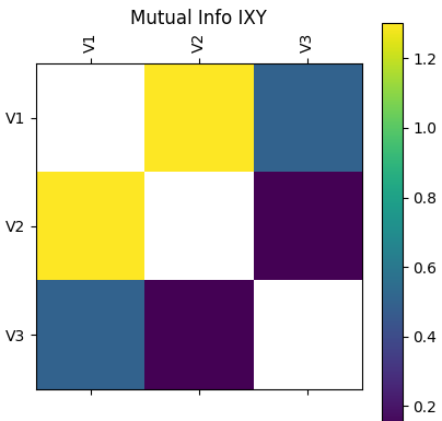
Create GMN network using the mutual information interaction matrix:
./CreateNetwork.py -i Lorenz3D_4k_iMatrix_MI.csv -t V3 -d 3 -o Lorenz3D_4k_Network_MI.pkl -v -P -as 30 -fs 26 -ns 200
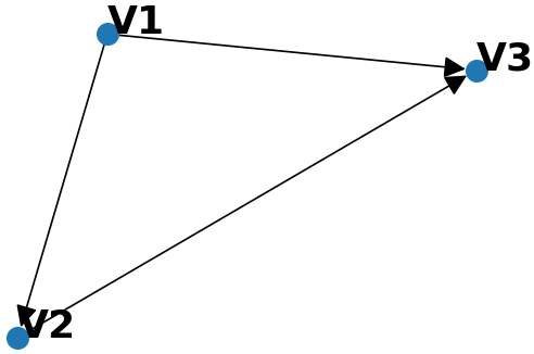
Examine GMN network:
from pickle import load

with open('Lorenz3D_4k_Network_MI.pkl', 'rb') as f:
     network = load(f)

network['Map']
### {'V3': ['V1', 'V2'], 'V1': [], 'V2': ['V1']}
network['Graph'].nodes
### NodeView(('V2', 'V3', 'V1'))
[_ for _ in network['Graph'].predecessors('V3')]
### ['V2', 'V1']
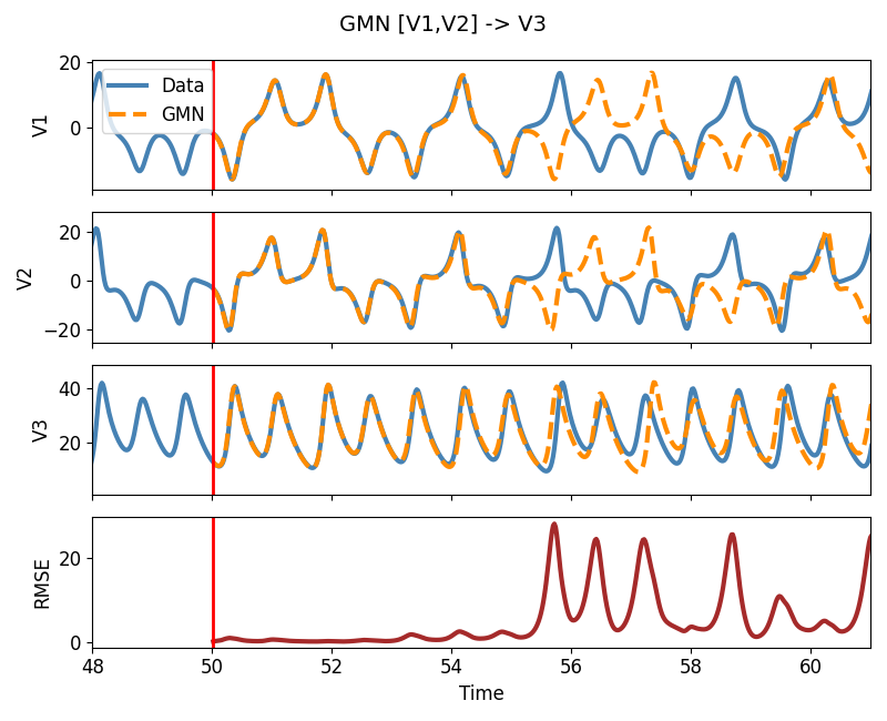
Run GMN without a config file using the GMN application RunNoConfig.py. Parameters: E=3, tau=-7, taget node V3, GMN network file Lorenz3D_4k_Network_MI.pkl, data file Lorenz3D_4k.csv. Start generation at index 2000, generate 1000 values.
./RunNoConfig.py -pS 2000 -pL 1000 -PT time -tn V3 \
-nf Lorenz3D_4k_Network_MI.pkl -nd ../data/Lorenz3D_4k.csv -E 3 \
-tau -7 -o GMN_Lorenz_E3_tau-7_pS_2000_pL_1000.csv
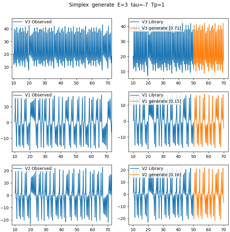
Plot generated dynamics and RMSE with PlotGMN.py application.
./PlotGMN.py
The ESN class is contained in ESN/ESN.py. The application wrapper ESN/RunESN.py is a command line interface to run the ESN.
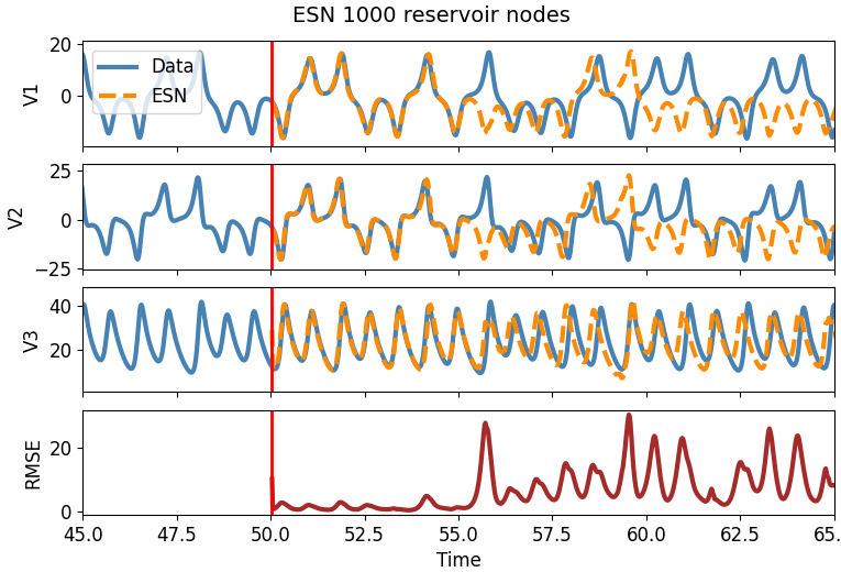
Run ESN on Lorenz'63 with 1000, 2000, 3000 nodes. Train ESN on first 2000 points, generate 1000 points.
cd ../ESN
./RunESN.py -R 500 -dg 3 -t 1 2000 -e 2001 3000 -i ../data/Lorenz3D_4k.csv \
-o ESN_R500_Lorenz3D_pS_2000_pL_1000.csv

./RunESN.py -R 1000 -dg 3 -t 1 2000 -e 2001 3000 -i ../data/Lorenz3D_4k.csv \
-o ESN_R1000_Lorenz3D_pS_2000_pL_1000.csv

./RunESN.py -R 2000 -dg 3 -t 1 2000 -e 2001 3000 -i ../data/Lorenz3D_4k.csv \
-o ESN_R2000_Lorenz3D_pS_2000_pL_1000.csv
Plot 1000 node generated dynamics and RMSE.
../GMN/PlotGMN.py -d ../data/Lorenz3D_4k.csv -i ESN_R1000_Lorenz3D_pS_2000_pL_1000.csv -g ESN -dv V1 V2 V3 -gv V1_ V2_ V3_ -t "ESN 1000 reservoir nodes" --xlim 45 65
cd ..
from pandas import read_csv
import matplotlib.pyplot as plt
from mpl_toolkits.mplot3d import Axes3D

gmnLorenz = read_csv('GMN/GMN_Lorenz_E3_tau-7_pS_2000_pL_1000.csv')
esnR500   = read_csv('ESN/ESN_R500_Lorenz3D_pS_2000_pL_1000.csv')
esnR1000  = read_csv('ESN/ESN_R1000_Lorenz3D_pS_2000_pL_1000.csv')
esnR2000  = read_csv('ESN/ESN_R2000_Lorenz3D_pS_2000_pL_1000.csv')

fig = plt.figure()
ax1 = fig.add_subplot(2, 2, 1, projection='3d')
ax2 = fig.add_subplot(2, 2, 2, projection='3d')
ax3 = fig.add_subplot(2, 2, 3, projection='3d')
ax4 = fig.add_subplot(2, 2, 4, projection='3d')

ax1.set_title( 'GMN' )
ax2.set_title( 'ESN 500' )
ax3.set_title( 'ESN 1000' )
ax4.set_title( 'ESN 2000' )

ax1.plot( gmnLorenz['V1'], gmnLorenz['V2'], gmnLorenz['V3'] )
ax2.plot( esnR500 ['V1_'], esnR500 ['V2_'], esnR500 ['V3_'] )
ax3.plot( esnR1000['V1_'], esnR1000['V2_'], esnR1000['V3_'] )
ax4.plot( esnR2000['V1_'], esnR2000['V2_'], esnR2000['V3_'] )
plt.show()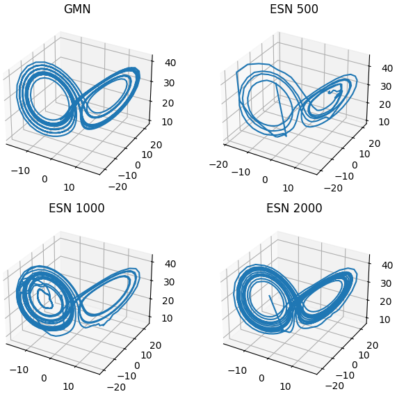
from pandas import read_csv
import matplotlib.pyplot as plt
import matplotlib.mlab as mlab

gmnLorenz = read_csv('GMN/GMN_Lorenz_E3_tau-7_pS_2000_pL_1000.csv')
esnR500   = read_csv('ESN/ESN_R500_Lorenz3D_pS_2000_pL_1000.csv')
esnR1000  = read_csv('ESN/ESN_R1000_Lorenz3D_pS_2000_pL_1000.csv')
esnR2000  = read_csv('ESN/ESN_R2000_Lorenz3D_pS_2000_pL_1000.csv')

nFFT    = 300
win     = mlab.window_hanning # mlab.window_none # mlab.window_hanning
overlap = 50
deltaT  = (gmnLorenz.loc[1,'Time'] - gmnLorenz.loc[0,'Time']).round(5)
fs      = 1 / deltaT

fig0, ax0 = plt.subplots(1, 1)
ax0.psd( esnR1000.loc[50:,'V1'], NFFT = nFFT, Fs = fs,
         window = win, noverlap = overlap, label = 'V1', lw = 3 )
ax0.psd( gmnLorenz.loc[100:,'V1'], NFFT = nFFT, Fs = fs,
         window = win, noverlap = overlap, label = 'GMN', lw = 2 )
ax0.psd( esnR500.loc[50:,'V1_'], NFFT = nFFT, Fs = fs,
         window = win, noverlap = overlap, label = 'ESN 500', lw = 2 )
ax0.psd( esnR1000.loc[50:,'V1_'], NFFT = nFFT, Fs = fs,
         window = win, noverlap = overlap, label = 'ESN 1k', lw = 2 )
ax0.psd( esnR2000.loc[50:,'V1_'], NFFT = nFFT, Fs = fs,
         window = win, noverlap = overlap, label = 'ESN 2k', lw = 2 )
ax0.legend()
plt.show()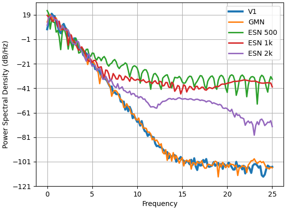
Compute interaction matrix with GMN InteractionMatrix.py application
cd GMN
./InteractionMatrix.py -d ../data/Fly80XY_norm_1061.csv -rhoDiff -oc Fly80_iMatrix -E 7 -P
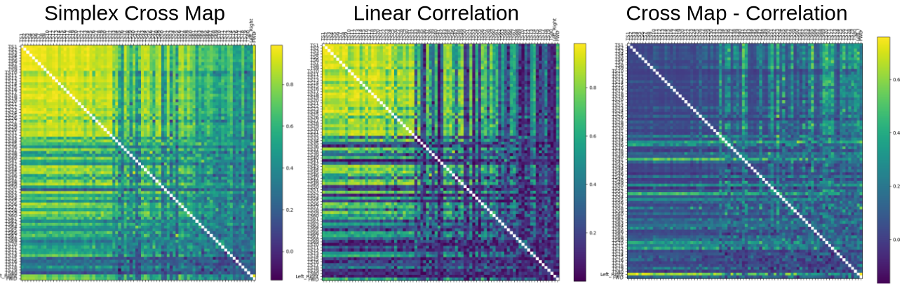
./CreateNetwork.py -i Fly80_iMatrix_rhoDiff.csv -d 5 -t FWD -x Left_Right -o Fly_Network_rhoDiff_D5_T0.23.pkl -T 0.23 -v
from pickle import load
import matplotlib.pyplot as plt
import networkx as nx

with open('Fly_Network_rhoDiff_D5_T0.23.pkl', 'rb') as f:
     network = load(f)

print( network['Map'] )

G = network['Graph']

nx.draw(G,with_labels=True,alpha=0.7,font_size=16,
        node_color='lightblue',font_weight='bold',
        pos=nx.arf_layout(G))

plt.show()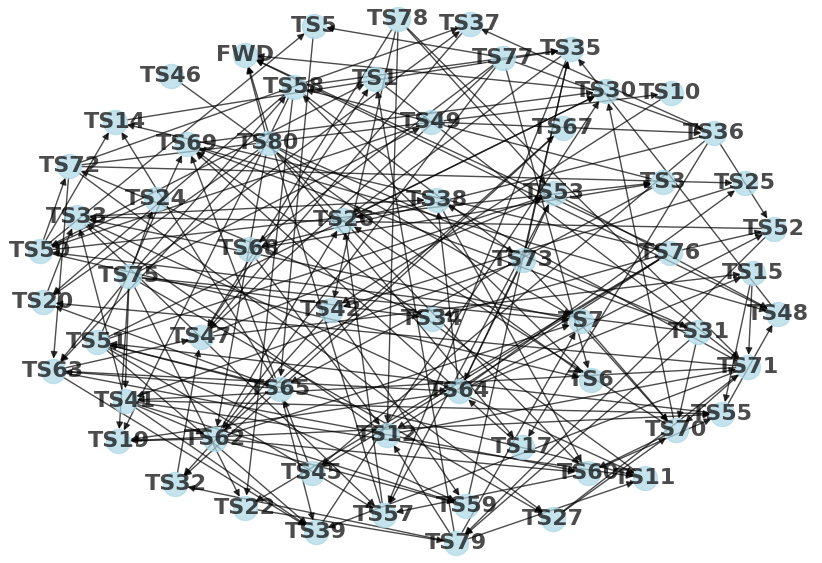
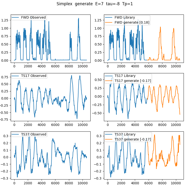
Run GMN on target node FWD with Tp 1 -E 7 -tau -8
./RunNoConfig.py -pS 580 -pL 480 -PT index -tn FWD \
-nf Fly_Network_rhoDiff_D5_T0.23.pkl \
-nd ../data/Fly80XY_norm_1061.csv -PT time -nn "Fly 80 : FWD" \
-Tp 1 -E 7 -tau -8 -do GMN_Fly80_1061_rhoDiff_D5_E7_tau-8.csv \
-PC FWD TS17 TS37 -P
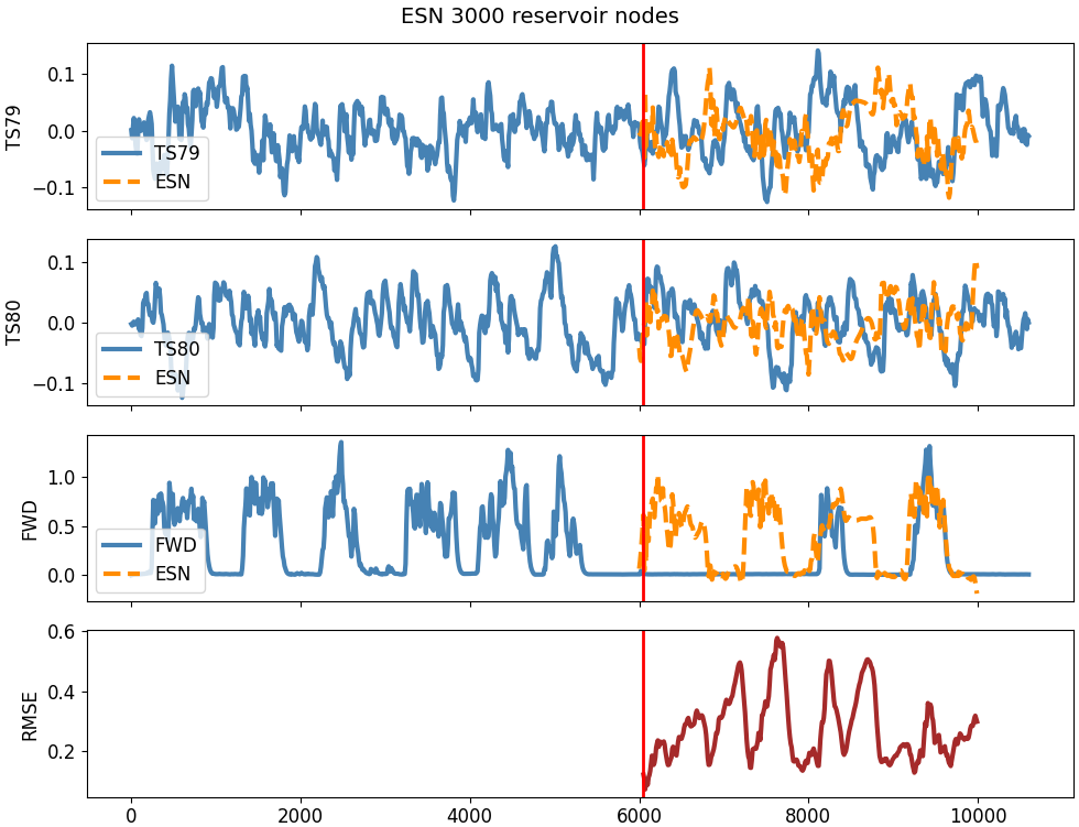
3000 node ESN to generate FWD : Same TS input as GMN with network Fly80_norm_rhoDiff_Network_D4.pkl
cd ../ESN

./RunESN.py -i ../data/Fly80XY_norm_1061.csv -sr 0.9 -lr 0.5 -time index \
-iv TS1 TS2 TS3 TS4 TS5 TS6 TS7 TS8 TS9 TS10 TS11 TS12 TS13 TS14 TS15 TS16 \
TS17 TS18 TS19 TS20 TS21 TS22 TS23 TS24 TS25 TS26 TS27 TS28 TS29 TS30 TS31 \
TS32 TS33 TS34 TS35 TS36 TS37 TS38 TS39 TS40 TS41 TS42 TS43 TS44 TS45 TS46 \
TS47 TS48 TS49 TS50 TS51 TS52 TS53 TS54 TS55 TS56 TS57 TS58 TS59 TS60 TS61 \
TS62 TS63 TS64 TS65 TS66 TS67 TS68 TS69 TS70 TS71 TS72 TS73 TS74 TS75 TS76 \
TS77 TS78 TS79 TS80 FWD -t 1 600 -b 5 -dg 7 -e 600 1000 -R 3000 \
-o ESN_Fly80_1061.csv -P
cd ..
from pandas import read_csv
import matplotlib.pyplot as plt

gmn = read_csv('GMN/GMN_Fly80_1061_rhoDiff_D5_E7_tau-8.csv').iloc[:420,:]
esn = read_csv('ESN/ESN_Fly80_1061.csv')

ax = esn.plot('index','FWD',lw=2)   # FWD data
gmn.plot('index','FWD',ax=ax,lw=2,label='GMN')  # GMN
esn.plot('index','FWD_',ax=ax,lw=2,label='ESN') # ESN
plt.show()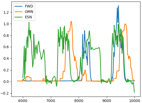
Compute interaction matrix with pyEDM CCM_Matrix.py application. Note this is an example matrix computed with a fixed embedding dimension E=10.
cd GMN
./CCM_Matrix.py -i ../data/J16_2021-06-05_epoch_8_1_Hz.csv -E 10 -of CCMTensor_J16_2021-06-05_epoch_8_1_Hz.npz -b 2000 -log -z 5 -v
Compute converged CCM based on CCM slope over library sizes
from CCM_Matrix import PlotMatrix
from numpy import load, nan

_ccm = load('CCMTensor_J16_2021-06-05_epoch_8_1_Hz.npz')
cmap1079 = _ccm['tensor'][:,:,3].copy() # Cross map matrix L=1079
columns  = _ccm['columns']
slope    = _ccm['slope']

PlotMatrix(cmap1079,columns,title='CCM J16 L=1078',figsize=(6,6), vmin=0.)
PlotMatrix(slope,columns,title='CCM Slope J16',figsize=(6,6), vmin=0.,vmax=0.3)

cmap1079[slope<0.1] = nan

PlotMatrix(cmap1079,columns,title='CCM J16',figsize=(6,6),vmin=0.3,vmax=0.8)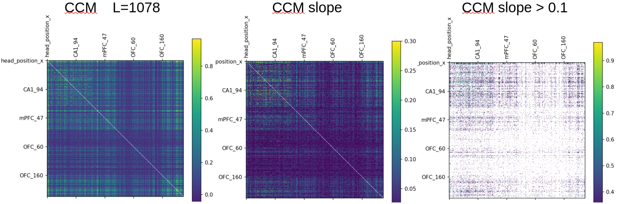
./CreateNetwork.py -i ../data/CCM_Converged_J16_2021-06-05_epoch_8_1_Hz.feather -df ../data/numDrivers_DF.feather -t head_position_x -x head_position_y head_velocity_x head_velocity_y head_speed head_orientation -o GMN_RatPosX_EDim_T0.6_CCM_Network.pkl -T 0.6
from pickle import load
import networkx as nx

with open('GMN_RatPosX_EDim_T0.6_CCM_Network.pkl','rb') as f:
        gmn = load(f)

G = gmn['Graph']

nx.draw( G, with_labels=True, alpha=0.7, font_size=16, node_color='lightgray',
         font_weight='bold', pos=nx.arf_layout(G)); plt.show()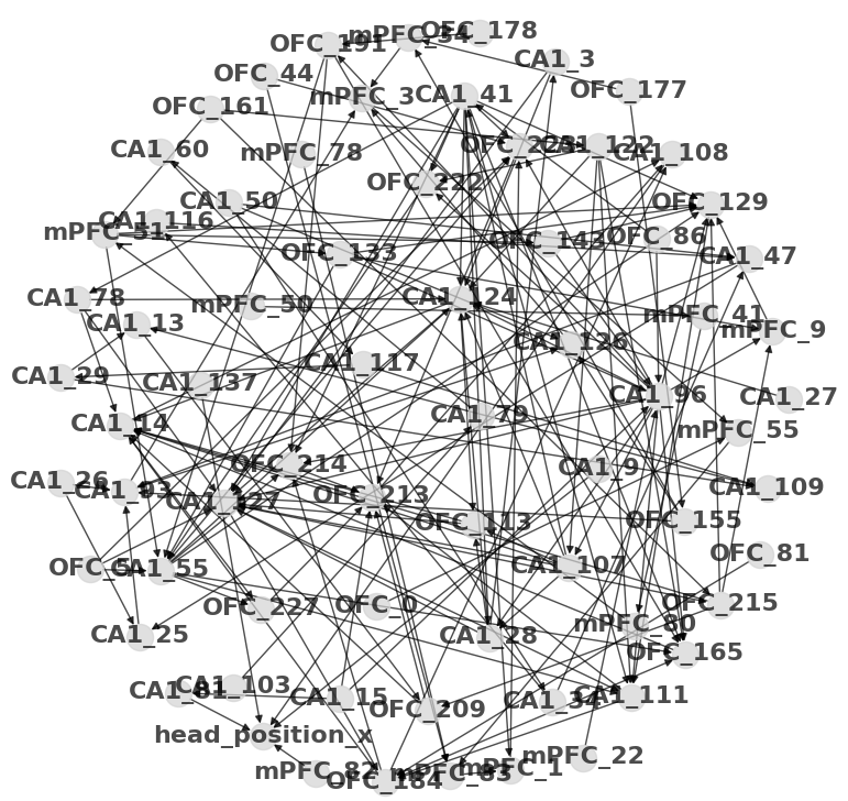
./RunNoConfig.py -E 7 -tau -7 -pS 1197 -pL 600 -tn head_position_x -nf GMN_RatPosX_EDim_T0.6_CCM_Network.pkl -nd ../data/J16_2021-06-05_epoch_8_1_Hz.csv -do RatJ16_PosX_EDim_T0.6_DataOut.feather
Plot observed and generated head_position_x
from pandas import read_feather, read_csv
from matplotlib import pyplot as plt

df = read_feather('RatJ16_PosX_EDim_T0.6_DataOut.feather')
data = read_csv('../data/J16_2021-06-05_epoch_8_1_Hz.csv')
dataX = data.iloc[-600:,:]['head_position_x']
df['head_position_x_obs'] = dataX.to_numpy()

ax = df.plot( x='time_bin_center', y=['head_position_x_obs','head_position_x'],
         lw=2, subplots=True )
ax[0].legend(['Observed head_position_x'])
ax[1].legend(['GMN head_position_x'])
plt.tight_layout()
plt.show()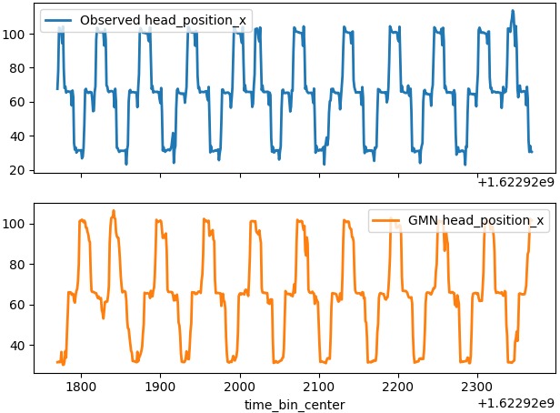
cd ../ESN

### NOTE: ESN with 50,000 nodes required ~4.5 hours on AMD EPYC 7742 64-Core Processor 1500.000 MHz

./RunESN.py -i ../data/J16_2021-06-05_epoch_8_1_Hz.csv -time time_bin_center -vf ../data/Rat_J16_nodes_EDim.csv -vn "./GMNet_PosX_EDim_T0.6.pkl" -t 1 600 -e 601 1190 -lr 0.5 -R 50000 -o ESN_RatJ16_T0.6_lr0.5_R50k_Out.csv
Plot observed and generated head_position_x
from pandas import read_csv
from matplotlib import pyplot as plt

df = read_csv('ESN_RatJ16_T0.6_lr0.5_R50k_Out.csv')

ax = df.plot( x='time_bin_center', y=['head_position_x','head_position_x_'],
         lw=2, subplots=True )
ax[0].legend(['Observed head_position_x'])
ax[1].legend(['ESN head_position_x'])
plt.tight_layout()
plt.show()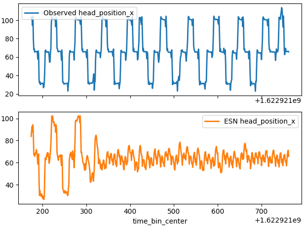
Comparison of crossformer with GMN.
Compute CCM interaction matrix of ETTh1 crossformer data.
./InteractionMatrix.py -d ../data/ETTh1.csv -cr 10 -cz 1000 -E 7 -P -ccm -v -s 50 -C 0.05 -oc ETTh1_iMatrix
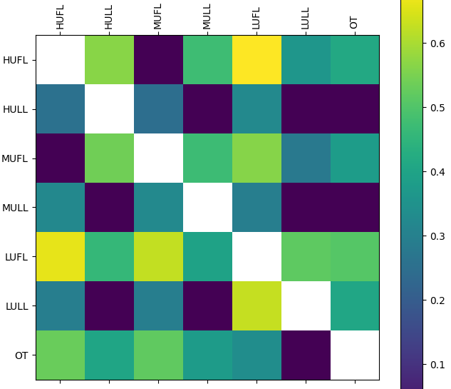
Create GMN network for the ETTh1 crossformer data.
./CreateNetwork.py -i ETTh1_iMatrix_CCM.csv -t OT -d 7 -P -l spring -nc lightblue -lw 2 -as 18 -fs 20 -ns 200 -o ETTh1_GMN_iMatrix_CCM.pkl
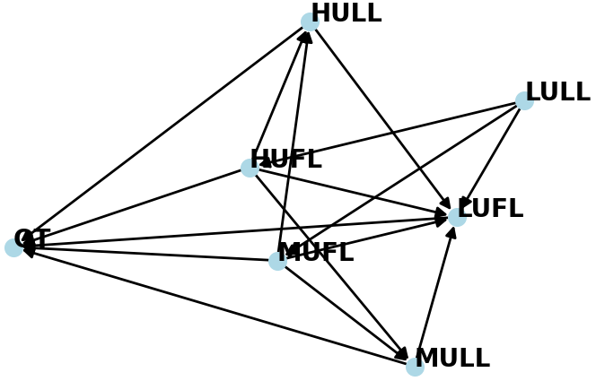
Run GMN in forecast mode to compare with crossformer which is not generative.
./RunNoConfig.py --mode forecast -tn OT -nf ETTh1_GMN_iMatrix_CCM.pkl -nd ../data/ETTh1.csv -E 5 -l "8000 11500" -p "11500 12220" -do ETTh1_GMN_iMatrix_CCM_DataOut.csv -v
Plot GMN results
from pandas import to_datetime, concat
data = read_csv('../data/ETTh1.csv')
data['date'] = to_datetime(data['date'])

df = read_csv('ETTh1_GMN_iMatrix_CCM_DataOut.csv')

df['date']=to_datetime(df['date'])
df.columns = ['date']+['GMN_'+s for s in df.columns[1:]]

# Subset data to match df from GMN forecast
mask = data['date'].isin( df['date'] )
data_ = data.loc[mask,:]

# Concat data_ and df (with renamed columns)
df_ = concat( [ data_.reset_index(drop=True),
                df.iloc[:,1:].reset_index(drop=True) ], axis='columns' )

# Error strings
from pyEDM import ComputeError
errD = {}
err = ComputeError(df_['OT'], df_['GMN_OT'])
errD[0] = f'rho {err['rho']:.2f}  RMSE {err['RMSE']:.2f}  CAE {err['CAE']:.1f}'
err = ComputeError(df_['MUFL'], df_['GMN_MUFL'])
errD[1] = f'rho {err['rho']:.2f}  RMSE {err['RMSE']:.2f}  CAE {err['CAE']:.1f}'
err = ComputeError(df_['HULL'], df_['GMN_HULL'])
errD[2] = f'rho {err['rho']:.2f}  RMSE {err['RMSE']:.2f}  CAE {err['CAE']:.1f}'

fig,axs = plt.subplots(nrows = 3, ncols = 1, sharex = True,
                       tight_layout = True, figsize = (6,6.5) )
df_.plot(y=['OT','GMN_OT'],    lw=2,ax=axs[0])
df_.plot(y=['MUFL','GMN_MUFL'],lw=2,ax=axs[1])
df_.plot(y=['HULL','GMN_HULL'],lw=2,ax=axs[2])

for i, ax in enumerate( axs ) :
    ax.text( 0.2, 0.88, errD[i], transform = ax.transAxes, fontsize = 12,
             bbox = dict(facecolor='white', linewidth=0,  alpha=1.0) )
    ax.tick_params(axis='both', labelsize=10)
    ax.legend(fontsize=12, loc='lower left')

plt.show()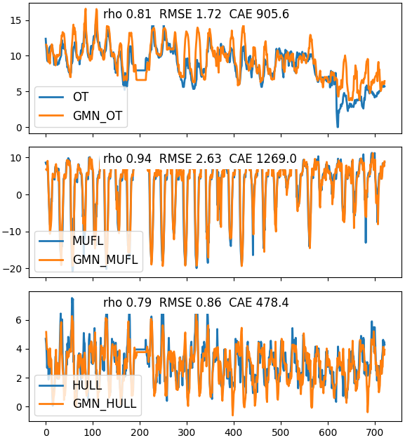
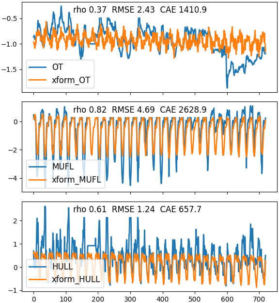
Download crossformer. Run on ETTh1 data to forecast 720 points with the main_crossformer.py application.
python main_crossformer.py --data ETTh1 --in_len 720 --out_len 720 --seg_len 24 --learning_rate 1e-5 --itr 5 --save_pred

cd results # In Crossformer
cd Crossformer_ETTh1_il720_ol720_sl24_win2_fa10_dm256_nh4_el3_itr4
Crossfomer result stored here in local Crossformer/
# Plot Crossformer results : rows 11520:12240 of ETTh1
df = read_csv('dfx0_ETTh1_il720_ol720.csv', index_col = 0)

# Observed data
data = read_csv('../data/ETTh1.csv')

# Crossformer standardises every column with a StandardScaler fit on the
# ETTh1 train split (the first 8640 rows) : x_scaled = (x - mu) / sigma.
# Both the observed (OT, MUFL...) and predicted (xform_*) columns of df are
# in that scaled space.  Invert it to recover the original units so RMSE and
# CAE are directly comparable to GMN, whose predictions are observed
# amplitudes.  Since the transform is affine, |err| scales by sigma alone.
columns = ['HUFL','HULL','MUFL','MULL','LUFL','LULL','OT']
train   = data.loc[ :8639, columns ]
mu      = train.mean()
sigma   = train.std( ddof = 0 )  # sklearn StandardScaler uses ddof = 0

# Error strings
from pyEDM import ComputeError
def ErrString( column ) :
    '''Un-scale Crossformer observed : predictions, then compute error'''
    obs  = df[ column ]            * sigma[ column ] + mu[ column ]
    pred = df[ 'xform_' + column ] * sigma[ column ] + mu[ column ]
    err  = ComputeError( obs.values, pred.values )
    errStr = f"rho {err['rho']:.2f}  RMSE {err['RMSE']:.2f}  " +\
             f"CAE {err['CAE']:.1f}"
    return errStr

errD = {}
errD[0] = ErrString( 'OT'   )
errD[1] = ErrString( 'MUFL' )
errD[2] = ErrString( 'HULL' )

# Plot the Crossformer output as-is, in the scaled space it is returned in.
# Only the error metrics are un-scaled, for comparison against GMN.
fig,axs = plt.subplots(nrows = len(errD), ncols = 1, sharex = True,
                       tight_layout = True, figsize = (6,6.5) )
df.plot(y=['OT','xform_OT'],    lw=2,ax=axs[0])
df.plot(y=['MUFL','xform_MUFL'],lw=2,ax=axs[1])
df.plot(y=['HULL','xform_HULL'],lw=2,ax=axs[2])

for i, ax in enumerate( axs ) :
    ax.text( 0.2, 0.88, errD[i], transform=ax.transAxes, fontsize=12,
             bbox = dict(facecolor='white', linewidth=0,  alpha=1.0) )
    ax.tick_params(axis='both', labelsize=10)
    ax.legend(fontsize=12, loc='lower left')

plt.show()