lonkit: Local Optima Networks in Python

lonkit is a Python library for constructing, analyzing, and visualizing Local Optima Networks (LONs) for both continuous and discrete optimization problems. LONs provide a powerful way to understand the structure of fitness landscapes, revealing how local optima are connected and how difficult it may be to find global optima.

Documentation: helix-agh.github.io/lonkit

Features

• LON Construction: Local Optima Networks as igraph graphs generated from sampled data, including Compressed Monotonic LONs (CMLONs).
• Continuous landscape exploration: Configurable Basin-Hopping algorithm for data sampling, with automatic step-size estimation and parallelization.
• Discrete landscape exploration: Iterated Local Search sampler, with parallelization, built-in problems (OneMax, NK Landscape, Number Partitioning) and classes to define custom problem instances.
• Landscape metrics: Funnel analysis, neutrality, global and sink strength, plus search performance (success rate, deviation from the known optimum).
• Visualization: Configurable 2D and 3D LON plots, and animated rotating GIFs.

Installation

pip install lonkit

Exporting 3D plots to images or GIFs also requires Chrome/Chromium. If it is not installed, run kaleido_get_chrome after installing lonkit. See the installation guide.

Or install from source:

git clone https://github.com/helix-agh/lonkit.git
cd lonkit
pip install -e .

Quick Start

import numpy as np
from lonkit import compute_lon, LONVisualizer, BasinHoppingSamplerConfig

# Define an objective function
def rastrigin(x: np.ndarray) -> float:
    return 10 * len(x) + np.sum(x**2 - 10 * np.cos(2 * np.pi * x))

# Construct the LON
config = BasinHoppingSamplerConfig(
    n_runs=20,
    n_iter_no_change=500,
    seed=42
)
lon = compute_lon(
    rastrigin,
    dim=2,
    lower_bound=-5.12,
    upper_bound=5.12,
    config=config
)

metrics = lon.compute_metrics()
print(f"Number of funnels: {metrics['n_funnels']}")
print(f"Global funnels: {metrics['n_global_funnels']}")

# Visualize
viz = LONVisualizer()
viz.plot_2d(lon, output_path="lon_2d.png")
viz.plot_3d(lon, output_path="lon_3d.png")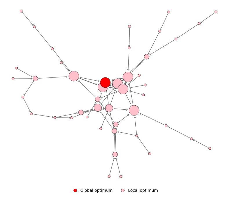

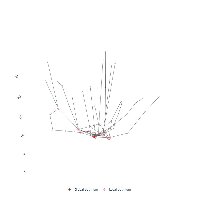plot_2d(lon)	plot_3d(lon): fitness on the Z-axis

Nodes are local optima and edges are transitions between them, with node size and edge width growing with how often they were visited.

Compressed Monotonic LONs (CMLONs)

CMLONs are a compressed representation where nodes with equal fitness that are connected get merged. This provides a cleaner view of the landscape's funnel structure.

# Convert LON to CMLON
cmlon = lon.to_cmlon()

# Analyze CMLON-specific metrics
cmlon_metrics = cmlon.compute_metrics()

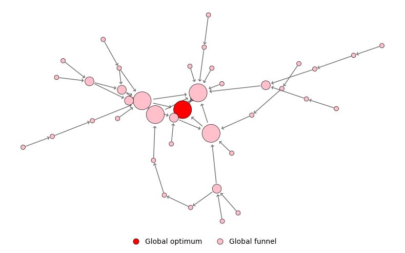LON: 45 optima	CMLON: 39 optima

Custom Sampling Configuration

from lonkit import BasinHoppingSampler, BasinHoppingSamplerConfig

config = BasinHoppingSamplerConfig(
    n_runs=50,                   # Number of independent runs
    n_iter_no_change=1000,       # Stop after this many consecutive non-improving perturbations
    step_size=0.05,              # Perturbation size
    step_mode="percentage",      # "percentage" or "fixed"
    coordinate_precision=4,      # Precision for identifying optima
    fitness_precision=None,      # Precision for fitness values (None = full double)
    seed=42                      # For reproducibility
)

sampler = BasinHoppingSampler(config)

# Define search domain
domain = [(-5.12, 5.12), (-5.12, 5.12)]

# Run sampling
result = sampler.sample(rastrigin, domain)
lon = sampler.sample_to_lon(result)

Discrete Optimization Problems

lonkit also supports Local Optima Networks for discrete optimization problems using Iterated Local Search (ILS). The library includes several built-in discrete problems for analysis: Number Partitioning, NK Landscape and OneMax.

from lonkit import NumberPartitioning, ILSSampler, ILSSamplerConfig, LONVisualizer

# Define problem instance
problem = NumberPartitioning(n=20, k=0.5, instance_seed=1)

# Configure and run ILS sampling
config = ILSSamplerConfig(n_runs=50, n_iter_no_change=100, seed=42)
sampler = ILSSampler(config)
result = sampler.sample(problem)

# Build LON and CMLON
lon = sampler.sample_to_lon(result)
cmlon = lon.to_cmlon()

# Compute metrics
print(lon.compute_metrics())
print(cmlon.compute_metrics())

# Visualize
viz = LONVisualizer()
viz.plot_2d(cmlon, output_path="npp_cmlon.png")

Custom Discrete Problems

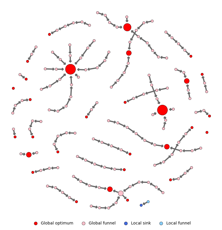
You can define your own discrete problem by subclassing DiscreteProblem. You can also extend built-in problems - for bitstring problems, extend BitstringProblem, which provides random_solution(), local_search(), perturb(), and solution_id() out of the box, so you only need to implement evaluate().

Documentation

The full documentation is at helix-agh.github.io/lonkit:

• Installation
• Quick Start
• Core Concepts: LONs and fitness landscapes
• Discrete Problems
• API Reference

References

• G. Ochoa, M. Tomassini, S. Vérel, C. Darabos. A Study of NK Landscapes' Basins and Local Optima Networks. GECCO 2008.
• G. Ochoa, N. Veerapen, F. Daolio, M. Tomassini. Understanding Phase Transitions with Local Optima Networks: Number Partitioning as a Case Study. EvoCOP 2017.
• J. Adair, G. Ochoa, K. M. Malan. Local Optima Networks for Continuous Fitness Landscapes. GECCO 2019 Companion.

Contributing

Contributions are welcome! Please feel free to submit a Pull Request.