modern-yolonas

A clean, minimal reimplementation of YOLO-NAS — no factories, no registries, no OmegaConf. Just PyTorch.

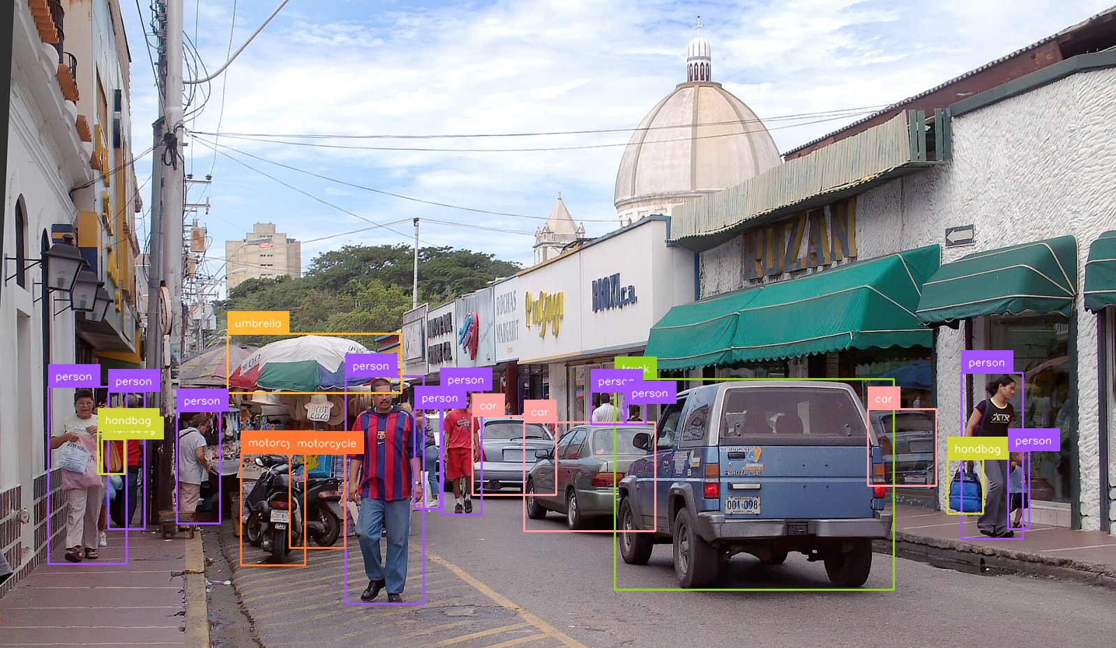
_{YOLO-NAS-L, confidence 0.40. Source photo by
Wilfredor, CC0.}

Live demo · Documentation · Changelog · Contributing · Issues

modern-yolonas is YOLO-NAS object detection rewritten so you can read the whole thing: a model variant is a function, a config is a dataclass, and there is no layer of indirection that exists only to be configurable. state_dict keys match super-gradients exactly, so the original pretrained COCO checkpoints load with strict=True.

Detections come back as supervision Detections, so every annotator, tracker, zone and metric in that ecosystem works on them out of the box. Training runs on Lightning, and the model exports to ONNX and OpenVINO — including a self-contained graph for Frigate.

🚀 Updates

[2026-09-18] v0.5.0 — training moved to PyTorch Lightning; quantization (yolonas quantize for PTQ, yolonas qat for QAT) on torch.ao.quantization FX graph mode; accuracy is now measured by this project rather than quoted; two mAP bugs and a mosaic bug fixed; license changed from MIT to Apache-2.0 for the source.
[2026-09-18] v0.4.0 — YoloNASDetector returns supervision.Detections, so results slice and plug into the supervision ecosystem directly.
[2026-02-05] v0.1 — initial release: S/M/L architectures, pretrained weight loading, training, COCO evaluation, and ONNX export.

🏆 Model Zoo

Box AP on COCO val2017, all 5000 images, and latency on the hardware named below. There is nothing to download by hand — yolo_nas_s(pretrained=True) and YoloNASDetector("yolo_nas_s") fetch and cache Deci's COCO checkpoints on first use (they carry Deci's own non-commercial terms — see License below). Pre-exported ONNX, OpenVINO IR and TensorRT engines are on the Hub.

Model	Input	Params	GFLOPs	AP	AP₅₀	dGPU _{TensorRT FP16}	CPU _{OpenVINO INT8}	iGPU _{OpenVINO INT8}
YOLO-NAS-S	320	19.05M	8.5	38.4	53.9	1.17 ms _{855 FPS}	5.19 ms _{193 FPS}	6.83 ms _{146 FPS}
YOLO-NAS-S	640	19.05M	33.9	47.3	64.4	2.12 ms _{472 FPS}	19.87 ms _{50 FPS}	12.04 ms _{83 FPS}
YOLO-NAS-M	320	51.18M	23.5	43.1	59.1	1.50 ms _{666 FPS}	12.03 ms _{83 FPS}	9.45 ms _{106 FPS}
YOLO-NAS-M	640	51.18M	94.2	51.3	68.3	4.19 ms _{239 FPS}	47.47 ms _{21 FPS}	25.49 ms _{39 FPS}
YOLO-NAS-L	320	66.98M	32.2	43.8	59.9	1.94 ms _{515 FPS}	15.56 ms _{64 FPS}	10.38 ms _{96 FPS}
YOLO-NAS-L	640	66.98M	129.0	52.0	69.1	5.41 ms _{185 FPS}	63.00 ms _{16 FPS}	32.07 ms _{31 FPS}

Every column is measured here, not quoted — regenerate the whole table with uv run examples/model_table.py and uv run examples/render_model_table.py. The full grid, across PyTorch / ONNX Runtime / OpenVINO / TensorRT and CPU / iGPU / dGPU, is in the runtime matrix.

How these numbers were measured, and what they do and do not mean

Latency is model forward only — no preprocessing, no NMS — batch 1, median of 30 runs after 8 discarded. FPS is its reciprocal on a single synchronous stream, not throughput: a pipeline that overlaps decode, transfer and inference reports more on the same hardware, and one that counts whole frames reports less, because preprocessing is excluded. Measured on an RTX 3060 Laptop / i7-12700H / Iris Xe, on mains power. The dGPU column is a TensorRT engine built natively on that card; an --hardware-compatible engine, which is the kind worth publishing, costs 16% at 320 and 8% at 640. Leaderboards that publish T4 TensorRT latency are not measuring the same thing, so those columns should not be read side by side.

320 costs about 9 AP, consistently across all three variants (−8.9 / −8.2 / −8.2), for roughly a quarter of the FLOPs. Worth knowing before choosing it: these weights were trained at 640, so this measures the resolution drop and not a model designed for 320. It also rules out an obvious-looking trade — YOLO-NAS-L at 320 is faster than YOLO-NAS-S at 640 on a CPU (15.6 ms against 19.9) and 3.5 AP worse, so the bigger model at lower resolution is not the free win the latency column alone suggests.

Accuracy is measured in FP32 with NMS at IoU 0.70, which a sweep found to be the optimum. postprocess still defaults to 0.65 for interactive use, where fewer overlapping boxes matters more than a tenth of AP.

The weights are Deci's pretrained COCO checkpoints, so this measures the architecture as reimplemented here, not weights trained by this project. Deci publishes 47.5 / 51.5 / 52.2, so roughly 0.2 is unaccounted for — the model table lists the protocol differences that were tested and ruled out, and does not guess at the rest. Numeric agreement with super-gradients is verified far more tightly: class scores are bit-identical.

📦 Installation

uv add modern-yolonas
# or
pip install modern-yolonas

Optional extras: [onnx], [openvino], [fiftyone], [benchmark], [serve], [demo], [tensorboard], [wandb].

⚡ Quick Start

YoloNASDetector picks CUDA when it is available and falls back to CPU, so the examples below run anywhere. Pass device="cuda", "cpu" or a torch.device to choose explicitly.

Detect objects in an image

import cv2
from modern_yolonas import YoloNASDetector

det = YoloNASDetector("yolo_nas_s")

image = cv2.imread("image.jpg")
detections = det(image)  # an sv.Detections

for box, score, name in zip(detections.xyxy, detections.confidence, detections.data["class_name"]):
    x1, y1, x2, y2 = box
    print(f"{name}: {score:.2f} [{x1:.0f}, {y1:.0f}, {x2:.0f}, {y2:.0f}]")

# Save annotated image
cv2.imwrite("output.jpg", det.annotate(image, detections))

Because the result is a supervision container, filtering is slicing:

from modern_yolonas import COCOClass

people = detections[detections.class_id == COCOClass.PERSON]
confident = detections[detections.confidence > 0.5]
big = detections[detections.box_area > 5000]

COCOClass is an IntEnum, so its members are ordinary ints — they just say which class they are. The ids describe the COCO taxonomy, so they apply to the pretrained checkpoints, not to a model fine-tuned on your own classes.

and it plugs straight into the rest of the ecosystem:

import supervision as sv

zone = sv.PolygonZone(polygon=my_polygon)
inside = detections[zone.trigger(detections)]

heatmap_annotator = sv.HeatMapAnnotator()
frame = heatmap_annotator.annotate(frame, detections)

Detect objects in a video

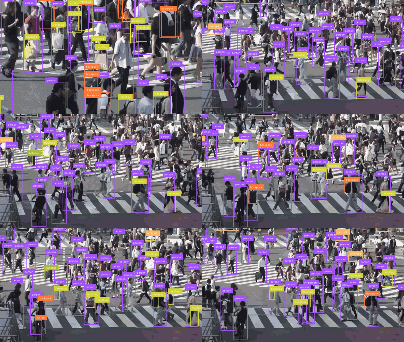
_{YOLO-NAS-L at confidence 0.25, ~70 detections per frame. Clip by
Basile Morin,
CC BY-SA 4.0 — so this
clip, unlike the rest of the repository, is CC BY-SA rather than Apache-2.0.}

from modern_yolonas import YoloNASDetector

det = YoloNASDetector("yolo_nas_s")

# Option 1: Write annotated video directly
stats = det.detect_video_to_file("input.mp4", "output.mp4")
print(f"{stats['total_detections']} detections across {stats['total_frames']} frames")

# Option 2: Iterate frames for custom logic
for frame_idx, frame, detections in det.detect_video("input.mp4"):
    print(f"Frame {frame_idx}: {len(detections)} objects")
    # detections.xyxy, .confidence, .class_id are numpy arrays
    # det.annotate(frame, detections) returns the annotated BGR frame

Live webcam detection

import cv2
from modern_yolonas import YoloNASDetector

det = YoloNASDetector("yolo_nas_s")

for frame_idx, frame, detections in det.detect_video(source=0):  # 0 = default camera
    cv2.imshow("YOLO-NAS", det.annotate(frame, detections))
    if cv2.waitKey(1) & 0xFF == ord("q"):
        break
cv2.destroyAllWindows()

Feature embeddings

The detector throws the backbone's representation away and keeps four numbers per object. YoloNASEmbedder keeps the representation — for image retrieval, near-duplicate search, clustering and re-identification. Nothing extra is trained: same weights, read one stage earlier.

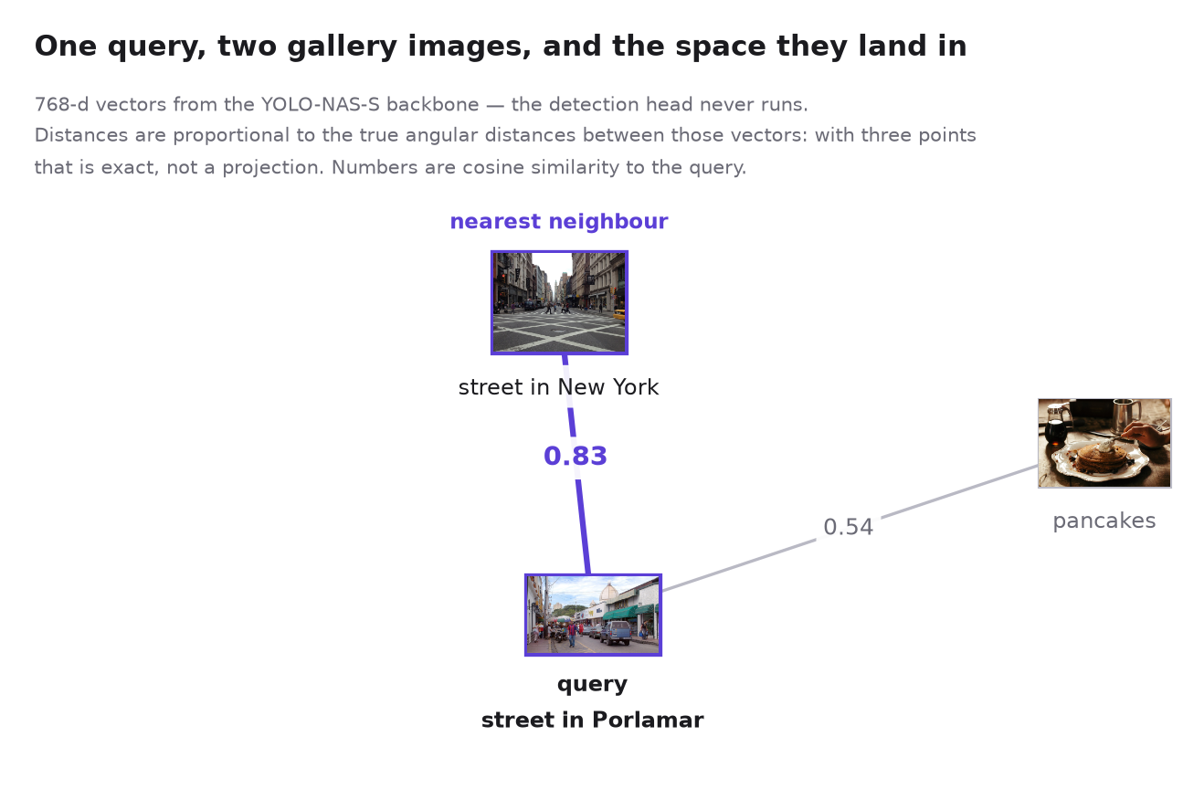
_{Regenerate with uv run examples/embedding_space_figure.py. Gallery photos by
Mike Petrucci and
Gabriel Gurrola, CC0.}

import numpy as np
from modern_yolonas import YoloNASEmbedder

embedder = YoloNASEmbedder("yolo_nas_s")

vector = embedder("image.jpg")                     # (768,) L2-normalized
gallery = embedder.embed_batch(["a.jpg", "b.jpg"]) # (2, 768)

# Both sides are normalized, so a dot product is the cosine similarity.
ranking = np.argsort(-(gallery @ vector))

Detections and embeddings in one pass

Detection and embedding share the whole network up to the head, so there is no reason to run the backbone twice. predict takes Task flags and gives you both:

from modern_yolonas import COCOClass, Task, YoloNASDetector

detector = YoloNASDetector("yolo_nas_s")
result = detector.predict(image, Task.DETECT | Task.EMBED | Task.EMBED_OBJECTS)

result.detections                       # sv.Detections
result.embedding                        # (768,) whole-image vector
result.detections.data["embedding"]     # (N, 768), one row per detection

# The per-object vectors live in `data`, so they follow the boxes through slicing:
people = result.detections[result.detections.class_id == COCOClass.PERSON]
people.data["embedding"]                # rows still aligned with people.xyxy

Task.EMBED_OBJECTS implies Task.DETECT; fields you did not ask for come back None. detector(image) still works — it is shorthand for predict(image, Task.DETECT).detections.

Raw feature maps, if you want to pool them yourself:

features = model.forward_features(x)   # c2 c3 c4 c5 (backbone) + p3 p4 p5 (neck)

All three shapes export to ONNX — --target embedding, --target combined, and --target objects, the last a self-contained graph with NMS inside it that emits detections [D, 7] and one vector per detection.

See the embeddings guide for layer choice and why the letterbox padding is excluded from pooling, and the export guide for the valid_region input the exported graphs take.

Track objects across a video

_{Boxes are coloured by track id, not by class, so an ID-swap shows as a colour change.
48 frames, 14 ids, 10 of them alive for at least half the clip.}

Tracking uses the same forward pass as detection — the per-object embeddings Deep HM-SORT associates on are the ones the detector already computed, so appearance-aware tracking costs one pass per frame rather than two.

from modern_yolonas import YoloNASDetector
from modern_yolonas.tracking import DeepHMSort

detector = YoloNASDetector("yolo_nas_s")
tracker = DeepHMSort()

for frame_index, frame, detections in detector.track_video("match.mp4", tracker):
    detections.tracker_id          # (N,) stable ids
    detections.data["embedding"]   # (N, 768) the vectors it associated on

# Or straight to a file, with ids drawn on
stats = detector.track_video_to_file("match.mp4", "tracked.mp4")
stats["unique_ids"]                # distinct objects the tracker believes it saw

A lost track stays findable for 2 seconds of video by default, counted with the clip's own frame rate rather than in frames, so the number means the same thing at 25 and 60 fps:

DeepHMSort()                       # 2 s — good default for open scenes
DeepHMSort(max_lost_seconds=10.0)  # a doorway, where people come back
DeepHMSort(max_lost_seconds=None)  # the paper: keep every tracklet, forever

The paper never discards a tracklet, which is right for a fixed camera on a closed pitch and wrong for a street — there the pool grows with every object ever seen. --keep-all-tracks restores the paper's behaviour.

Deep HM-SORT fuses the motion and appearance costs with their harmonic mean instead of taking the smaller one, which stops a lookalike from stealing an id on appearance alone, and it keeps every tracklet for the whole sequence so an object that leaves the frame and returns is re-identified rather than renumbered. It has no Kalman filter — Deep-EIoU drops it in favour of expanding the boxes before intersecting them.

The appearance vectors are a by-product of detection, not a re-identification model trained to tell two people apart, so the paper's HOTA numbers are not inherited here. Any (N, D) array in detections.data["embedding"] is associated on, so a purpose-trained model drops straight in — see the tracking guide.

Low-level model API

import torch
from modern_yolonas import yolo_nas_s

model = yolo_nas_s(pretrained=True).eval().cuda()
x = torch.randn(1, 3, 640, 640).cuda()
pred_bboxes, pred_scores = model(x)
# pred_bboxes: [1, 8400, 4] — x1y1x2y2 pixel coordinates
# pred_scores: [1, 8400, 80] — class probabilities

🖥️ CLI

Full reference: CLI docs.

# Detect in images
yolonas detect --model yolo_nas_s --source image.jpg --conf 0.25
yolonas detect --model yolo_nas_l --source images/ --output results/

# Detect in video
yolonas detect --model yolo_nas_s --source video.mp4 --output results/
yolonas detect --model yolo_nas_m --source video.mp4 --skip-frames 2 --conf 0.3

# Track objects across a video (Deep HM-SORT)
yolonas track --source match.mp4 --classes 0
yolonas track --source match.mp4 --fusion min                  # the Deep-EIoU baseline
yolonas track --source lobby.mp4 --max-lost-seconds 10          # remember people for longer

# Training
yolonas train --model yolo_nas_s --data /path/to/dataset --format yolo --epochs 100

# Evaluation
yolonas eval --model yolo_nas_s --data /path/to/coco --split val2017

# Export (needs the extras: pip install "modern-yolonas[onnx]" / [openvino])
yolonas export --model yolo_nas_s --format onnx --output model.onnx
yolonas export --model yolo_nas_s --format openvino --output model.xml

# Export feature embeddings, alone or beside the detections
yolonas export --model yolo_nas_s --target embedding --output embedding.onnx
yolonas export --model yolo_nas_s --target combined --output combined.onnx
yolonas export --model yolo_nas_s --target objects --output objects.onnx

# Export for Frigate (embeds preprocessing + NMS in the graph)
yolonas export --model yolo_nas_s --format onnx --target frigate
yolonas export --model yolo_nas_s --format openvino --target frigate --input-size 320

Frigate integration

The --target frigate export produces a self-contained model that accepts raw uint8 BGR input and outputs a flat [D, 7] tensor with [batch, x1, y1, x2, y2, confidence, class_id].

detectors:
  ov:
    type: openvino
    device: GPU

model:
  model_type: yolonas
  width: 320
  height: 320
  input_tensor: nchw
  input_pixel_format: bgr
  path: /config/model_frigate.xml

📚 Tutorials

Step-by-step notebooks in tutorials/:

Topic	Notebook	Description
Roboflow	`roboflow/01_explore_dataset.ipynb`	Download from Roboflow + explore
	`roboflow/02_finetune.ipynb`	Fine-tune + evaluate + visualize
FiftyOne	`fiftyone/01_explore_dataset.ipynb`	Load from FiftyOne Zoo + explore
	`fiftyone/02_finetune.ipynb`	Fine-tune + evaluate + visualize
	`fiftyone/03_embedding_space.ipynb`	Explore a YOLO-NAS embedding space + find duplicates
Export	`export_onnx.ipynb`	ONNX export from any checkpoint
Quantization	`quantization_ptq.ipynb`	Post-Training Quantization
	`quantization_qat.ipynb`	Quantization-Aware Training
Inference	`inference_onnx.ipynb`	ONNX Runtime inference

Examples

Start with the notebook — install, detect, visualize, and inspect the raw model output in one pass:

notebooks/quickstart.ipynb

Or the standalone scripts in examples/:

parity_check.py — verify this implementation matches super-gradients (writes docs/benchmarks/parity.md)
runtime_matrix.py — latency across PyTorch / ONNX Runtime / OpenVINO / TensorRT, CPU / Intel iGPU / NVIDIA dGPU, FP32 / FP16 / INT8 and every input size (writes docs/benchmarks/runtime_matrix.md)
runtime_accuracy.py — COCO AP for an exported artifact, so an INT8 file's accuracy is measured rather than assumed
export_zoo.py — pre-export every variant to every runtime and size, with a manifest
detect_image.py — run detection on a single image
detect_video.py — run detection on a video file
detect_webcam.py — live webcam detection
track_video.py — track a video with Deep HM-SORT and report whether the ids are fragmenting

🛠️ Development

uv sync --dev
uv run pre-commit install

uv run pytest tests/ -v
uv run ruff check src/ tests/

Contributions are welcome. Please read CONTRIBUTING.md — it lists the API design principles a change is reviewed against — and the Code of Conduct.

📄 License

Apache-2.0 — applies to the source code only. See LICENSE.

Pretrained weights notice: the pretrained COCO weights downloaded by this library (via pretrained=True) are provided by Deci AI and are subject to Deci's YOLO-NAS license, which restricts commercial use and redistribution. The Apache-2.0 license of this repository does not cover them. If you train your own weights from scratch, those are entirely yours.

🙏 Acknowledgments

This project is a clean-room reimplementation of the YOLO-NAS architecture originally developed by Deci AI and published in their super-gradients library (Apache-2.0). The model architecture, module structure and state_dict key naming were derived from the super-gradients source to enable pretrained weight compatibility.

It also builds directly on supervision, PyTorch Lightning and OpenVINO.

Thanks to everyone who has contributed — in particular Alan Neves, whose work on augmentations, metrics, gradient accumulation, the ONNX export path and super-gradients parity shaped much of the training stack.

⭐ Star History

📖 Citation

If you use modern-yolonas in your research or project, please cite it:

@software{condados2026modernyolonas,
  author       = {Condados, Luis and Neves, Alan},
  title        = {modern-yolonas: A Clean Reimplementation of YOLO-NAS},
  year         = {2026},
  url          = {https://github.com/CondadosAI/modern-yolonas},
  license      = {Apache-2.0}
}

Name		Name	Last commit message	Last commit date
.github		.github
configs		configs
docs		docs
examples		examples
notebooks		notebooks
spaces		spaces
src/modern_yolonas		src/modern_yolonas
tests		tests
tools		tools
tutorials		tutorials
.gitignore		.gitignore
.pre-commit-config.yaml		.pre-commit-config.yaml
.python-version		.python-version
CHANGELOG.md		CHANGELOG.md
CITATION.cff		CITATION.cff
LICENSE		LICENSE
README.md		README.md
ROADMAP.md		ROADMAP.md
SPONSORS.md		SPONSORS.md
mkdocs.yml		mkdocs.yml
pyproject.toml		pyproject.toml
uv.lock		uv.lock

Navigation Menu

Repository navigation

About

Repository files navigation

modern-yolonas

A clean, minimal reimplementation of YOLO-NAS — no factories, no registries, no OmegaConf. Just PyTorch.

🚀 Updates

🏆 Model Zoo

📦 Installation

⚡ Quick Start

Detect objects in an image

Detect objects in a video

Live webcam detection

Feature embeddings

Detections and embeddings in one pass

Track objects across a video

Low-level model API

🖥️ CLI

📚 Tutorials

Examples

🛠️ Development

📄 License

🙏 Acknowledgments

⭐ Star History

📖 Citation

About

Releases

Packages

Contributors

Languages

Latest commit

History

Folders and files

Repository files navigation

modern-yolonas

A clean, minimal reimplementation of YOLO-NAS — no factories, no registries, no OmegaConf. Just PyTorch.

🚀 Updates

🏆 Model Zoo

📦 Installation

⚡ Quick Start

Detect objects in an image

Detect objects in a video

Live webcam detection

Feature embeddings

Detections and embeddings in one pass

Track objects across a video

Low-level model API

🖥️ CLI

📚 Tutorials

Examples

🛠️ Development

📄 License

🙏 Acknowledgments

⭐ Star History

📖 Citation

About

Topics

Resources

Code of conduct

Contributing

Stars

Watchers

Forks

Releases

Packages

Contributors

Languages